 |
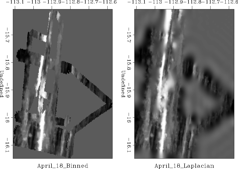
Figure 20 On the left, the SeaBeam data: the depth of the ocean under ship tracks; on the right, an interpolation with the Laplacian filter.
The next example is the SeaBeam dataset, a result of water bottom measurements from a single day of acquisition. This dataset has been used at the Stanford Exploration Project for benchmarking different strategies of data interpolation (, , , , , ). The left plot in Figure 20 shows the original data. The right plot shows the result of (unpreconditioned) missing data interpolation with the Laplacian filter. The result is unsatisfactory, because the Laplacian filter does not absorb the spatial frequency distribution of the input dataset. We judge the quality of an interpolation scheme by its ability to hide the footprints of the acquisition geometry in the final result.
 |
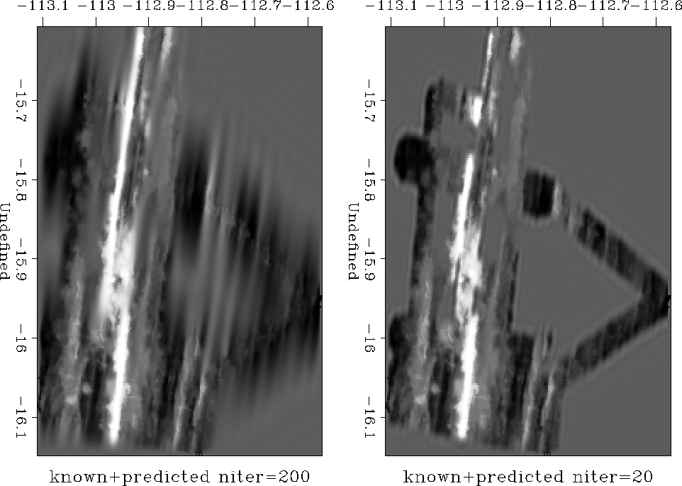
We can obtain a significantly better result (Figure 21) by replacing the Laplacian filter with a two-dimensional prediction-error filter (PEF) estimated from the input data. The result in the left plot of Figure 21 was obtained after 200 conjugate-gradient iterations. If we stop after 20 iterations, the output (the right plot in Figure 21) shows only a small deviation from the input data. Large areas of the image remain unfilled. At each iteration, the interpolation process progresses only to the length of the filter.
 |
![[*]](http://sepwww.stanford.edu/latex2html/movie.gif)
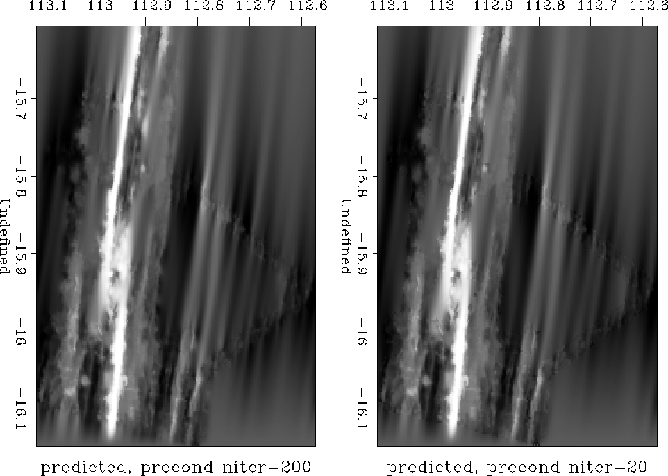
Inverting the PEF convolution with the help of the helix transform, we can now apply the inverse filtering operator to precondition the interpolation problem. As expected, the result after 200 iterations (the left plot in Figure 22) is similar to the result of the corresponding unpreconditioned interpolation. However, the output after just 20 iterations (the right plot in Figure 22) is already fairly close to the solution.
 |
![[*]](http://sepwww.stanford.edu/latex2html/movie.gif)