|
small-filter
Figure 4 A steering filter which annihilates dips of 22.5 degrees. | 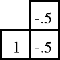 |
If we examine our desired model, it is apparent that the covariance function varies within at least two of our four patches (we can also see this in the covariance function of patch 2 and 4 of Figure 3). Therefore, it follows that we should get a better image by making smaller and smaller patches. Crawley (1998) showed that this is true when solving a data interpolation problem. Traditional methods for characterizing the model like PEFs and variograms can only grow so small before we have insufficient statistics to calculate them.
When our stationary assumption is valid, such as in regions one and four of Figure 3 the covariance matrix is fairly simple. We have a primary trend oriented along the dip of the velocity field that slowly dies out and a ringing effect due to the sinusoidal nature of our model. We would like to come up with a way to emulate the primary trend of the covariance matrix through minimal information.
To do this it is important to remember that our regularization operator should have the inverse spectrum of the covariance matrix. Therefore if the covariance function is primarily a dipping event, our regularization operator should be destroying that dip. Claerbout showed how to estimate the primary dip in a region and how to construct a filter that could destroy that dip. These small filters, which I refer to as steering filters can be as simple as a two or three point filter, Figure 4. A steering filter consists of a fixed `1' and one or more coefficients in the next column. The location of the filter coefficients in the second column determines the dip that the filter will destroy. Figure 5 is the inverse impulse response of Figure 4. Note how the general orientation of the impulse response is approximately the same as the covariance function below the lower unconformity.
|
small-filter
Figure 4 A steering filter which annihilates dips of 22.5 degrees. |  |
|
small-response
Figure 5 The impulse response of the inverse of Figure 4. | 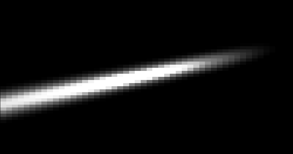 |
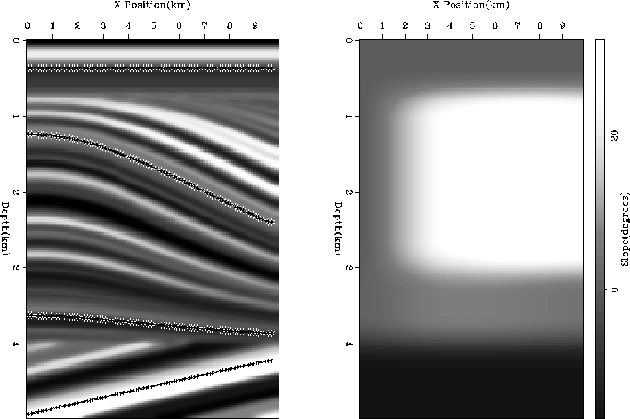
If we assume that velocity follows structure and we have some guesses at reflector position, we can use this information to build our steering filters. For this problem we will assume that we have the location of four reflectors, one above the top unconformity, two between the unconformities and one below the lower unconformity (left-panel of Figure 6). If we interpolate these dips to our entire model space we have all we need to construct a space-varying operator composed of steering filters. If we use this operator as our regularizer, we get Figure 7 as our interpolation result. The steering filters did a significantly better job than the isotropic regularizer.
 |
|
qdome-reg-cont
Figure 7 The result of using our steering filter operator as regularizer to the missing data problem. | 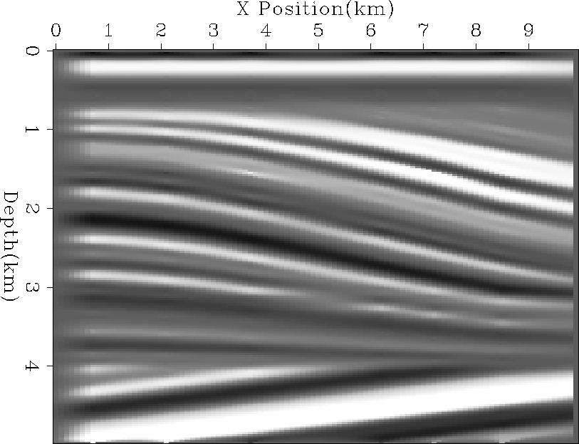 |