 |
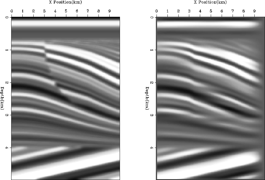
Figure 8 Left panel is a synthetic velocity model with the beds being offset by a listric fault. The right panel is the result of interpolating the model using steering filters.
Now let's move onto a model with discontinuities. Figure 8 is similar to Figure 1, with the exception that we now have a listric fault in the middle of the anticline structure. If we follow the same interpolation path as we did in the last section, the right panel of Figure 8 is our interpolation result.
 |
Instead of reproducing the fault we have created a model that smoothly changes from horizons on the left of the fault to the corresponding horizons to the right side of the fault. In many cases a smooth change is not only acceptable, but desirable (for example, ray-based methods require a smooth model). In other cases the smooth change is unrealistic and something we want to avoid (salt boundaries and some fault boundaries). Our interpolation fails at the fault because we are not correctly describing the covariance along the edge of the fault. The problem is that the covariance function at the edge of the fault is not symmetric. Along the left edge of the fault we have good correlation with points to the left but our correlation with points to the right our correlation is shifted. This asymmetric behavior is difficult to describe with steering filters.