In general, geophysical inverse problems (inverting for some
model (![]() ), given some (
), given some (![]() ),
while applying some operator (
),
while applying some operator (![]() ))
are ill-posed.
A classic example of this is the missing data problem Claerbout (1999).
The goal of
the missing data problem is to interpolate intelligently
between a sparse set of known points. For example, let's take
a synthetic velocity model with an upper horizontal reflector,
an anticline between two unconformities, and updipping layer
at the bottom of the model. Suppose
we have velocity measurements at several wells (Figure 1) and
you would like to interpolate it onto a regular 2-D mesh.
))
are ill-posed.
A classic example of this is the missing data problem Claerbout (1999).
The goal of
the missing data problem is to interpolate intelligently
between a sparse set of known points. For example, let's take
a synthetic velocity model with an upper horizontal reflector,
an anticline between two unconformities, and updipping layer
at the bottom of the model. Suppose
we have velocity measurements at several wells (Figure 1) and
you would like to interpolate it onto a regular 2-D mesh.
 |
The geophysicist might follow the approach described by
Claerbout (1999),
first interpolating the irregular data onto a regular mesh
by applying some type of binning operator, ![]() ,then defining a fitting goal that requires the model to fit
the data exactly at the known points (
,then defining a fitting goal that requires the model to fit
the data exactly at the known points (![]() ),
),
| |
(1) |
| |
(2) |
If
we don't have any other knowledge about our model,
an
isotropic operator like the Laplacian might be a logical choice for ![]() since it leads to the ``minimum energy'' solution.
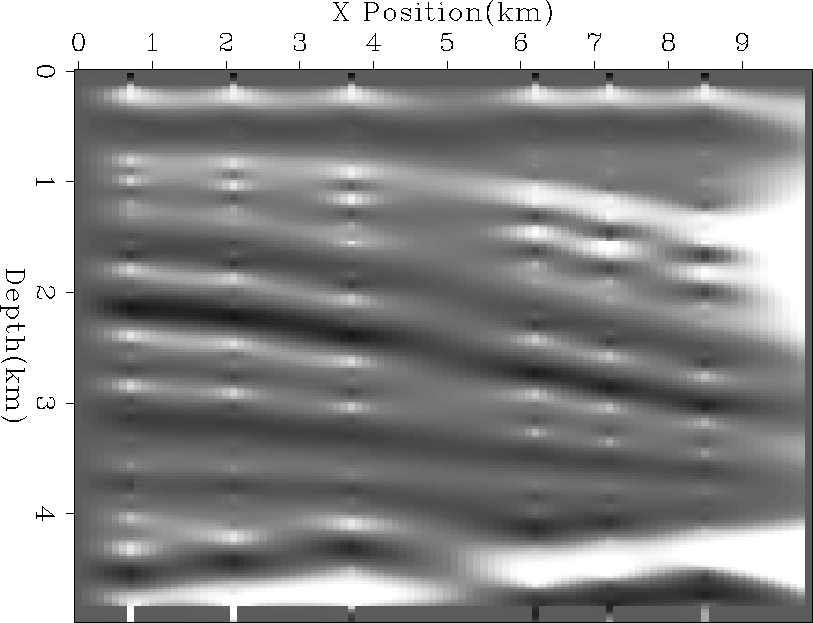
If I apply the fitting goals implied by (1) and
(2) for 200 iterations
using the Laplacian for
since it leads to the ``minimum energy'' solution.
If I apply the fitting goals implied by (1) and
(2) for 200 iterations
using the Laplacian for ![]() I get Figure 2.
The result is what
has been euphemistically referred to as
the `ice cream cone result' Brown (1998).
By spreading information
isotropically, the model goes smoothly from
our known points to some local average.
We see little to no continuation of layers,
which is generally a thoroughly unsatisfactory result.
I get Figure 2.
The result is what
has been euphemistically referred to as
the `ice cream cone result' Brown (1998).
By spreading information
isotropically, the model goes smoothly from
our known points to some local average.
We see little to no continuation of layers,
which is generally a thoroughly unsatisfactory result.
|
qdome-lap
Figure 2 Interpolation result after 200 iterations using an inverse Laplacian regularization operator. Note the edges effects at the top and bottom of the model due to using a internal convolution operator. |  |