|
|
|
|
Wave-equation migration velocity analysis for VTI media using optimized implicit finite difference |
 ,
,
 and
and
 . Anisotropic parameter
  relates the
vertical P-wave velocity
relates the
vertical P-wave velocity  with the NMO velocity
  , while the anellipticity parameter
  relates the horizontal
velocity
relates the horizontal
velocity  with the NMO velocity
.
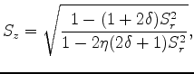
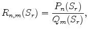
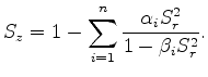
Shan (2009) suggests that the exact dispersion relationship 1 can be approximated by a rational
function
with the NMO velocity
.
Shan (2009) suggests that the exact dispersion relationship 1 can be approximated by a rational
function
 :
:
 , dispersion
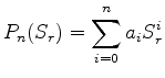
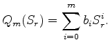
relationship 2 can be further split as follows:
, dispersion
relationship 2 can be further split as follows:
 and
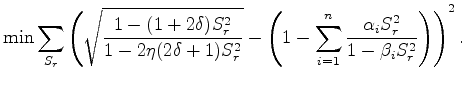
and  can be obtained by solving the least-square problem below:
 and
and
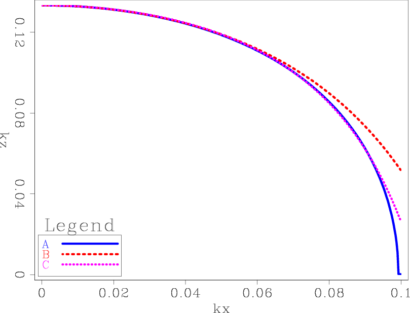
 . Curve A is the exact dispersion relation from Equation 1. Curve B is obtained
from a previous estimation by Ristow and Ruhl (1997), and curve C is obtained using the optimized coefficients. Apparently, the dispersion
relation using the optimized coefficients is a better approximation compared with the previous method which uses Taylor expansion and assumes
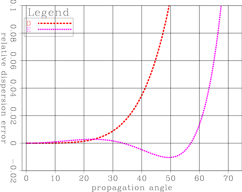
weak anisotropy. The relative errors between these two approximated curves and the exact dispersion curve are plotted in Figure 1(b).
Within a tolerance of 1% relative error in the dispersion relation, the optimized dispersion is accurate up to
. Curve A is the exact dispersion relation from Equation 1. Curve B is obtained
from a previous estimation by Ristow and Ruhl (1997), and curve C is obtained using the optimized coefficients. Apparently, the dispersion
relation using the optimized coefficients is a better approximation compared with the previous method which uses Taylor expansion and assumes
weak anisotropy. The relative errors between these two approximated curves and the exact dispersion curve are plotted in Figure 1(b).
Within a tolerance of 1% relative error in the dispersion relation, the optimized dispersion is accurate up to  , while the
Taylor approximation is only accurate up to
, while the
Taylor approximation is only accurate up to  .
.
|
|---|
|
kz1,err1
Figure 1. (a) Dispersion relation curves: A, exact dispersion relation curve from equation 1; B, approximated dispersion curve from weak anisotropy and Taylor expansion; C, approximated dispersion curve from optimization. (b) Relative dispersion error: D, relative error between B and A; E, relative error between C and A. |
|
|
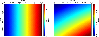
The tables for coefficients  and
and  for
ranging from 0
to
for
ranging from 0
to  and
ranging from
and
ranging from  to
to  are shown in Figure 2. In general, parameter
is more sensitive to the change in
than to the change in
.
Parameter
has similar sensitivities to both
and
.
are shown in Figure 2. In general, parameter
is more sensitive to the change in
than to the change in
.
Parameter
has similar sensitivities to both
and
.
|
|---|
|
coef
Figure 2. (a) Table for
and (b) table for
at discrete
and
locations.
|
|
|
|
|
|
|
Wave-equation migration velocity analysis for VTI media using optimized implicit finite difference |