|
|
|
|
Wave-equation migration velocity analysis for VTI media using optimized implicit finite difference |
 ,
which relates the perturbation in the anisotropic models (
,
which relates the perturbation in the anisotropic models (
 ) to
to the perturbation in the image (
) to
to the perturbation in the image ( ) and vice versa. Namely,
![$ {\bf m} = [v_v~\eta]$](img42.png) .
.
I refer the readers to Li and Biondi (2010) for a detailed derivation for the tomographic operator.
A different approximation to the exact dispersion relation leads to a different perturbed wave fields due to a perturbation in the model parameters. When the only available
data come from surface seismic surveys, parameter  is the least constrained (Plessix and Rynja, 2010; Li and Biondi, 2011b). Therefore, I assume the
model is perfectly
obtained from other sources of data and keep it fixed throughout the inversion. I will invert for
is the least constrained (Plessix and Rynja, 2010; Li and Biondi, 2011b). Therefore, I assume the
model is perfectly
obtained from other sources of data and keep it fixed throughout the inversion. I will invert for  and
and  in this study.
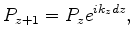
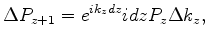
In the downward extrapolation, the wavefield at the next depth ( ) can be computed from the wavefield at the current depth (
 ) according to the following equation:
 ,
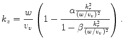
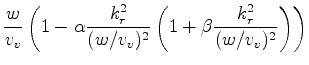
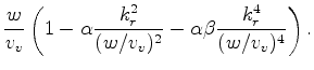
,  is the extrapolation distance in depth and
  can be obtained from the first-order approximation of the
dispersion relation 5:
can be obtained from the first-order approximation of the
dispersion relation 5:
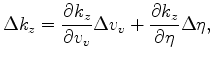
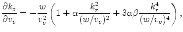
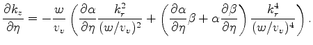
 and
and  are obtained by optimization, the derivatives in Equation 15
are obtained numerically by taking derivatives along the
axis in Figure 2. The tables of the derivatives of the
coefficients with respect to
are shown in Figure 3.
are obtained by optimization, the derivatives in Equation 15
are obtained numerically by taking derivatives along the
axis in Figure 2. The tables of the derivatives of the
coefficients with respect to
are shown in Figure 3.
|
|---|
|
dr-coef
Figure 3. (a) Table for  and (b) table for
 at background
and
locations.
at background
and
locations.
|
|
|
I test the implementation of the adjoint tomographic operator using this optimized implicit finite difference scheme in a homogeneous background VTI medium with
 km,
km,  and
and
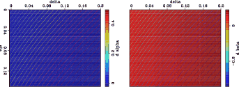
 . The synthetic data is produced by Born modeling with a horizontal reflector at the depth of 1500 km.
The input of the adjoint tomographic operator is a spike in the image space
. The synthetic data is produced by Born modeling with a horizontal reflector at the depth of 1500 km.
The input of the adjoint tomographic operator is a spike in the image space
 . The dominant frequency of the source wavelet is
 Hz, and the samplings in all directions are
  m.
m.
|
|---|
|
2dkernel
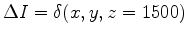
Figure 4. 2D impulse responses for vertical velocity (left column) and
(right column). Top row: zero offset impulse responses;
middle row: impulse responses when source-receiver offset is  km; bottom row: summation of the two rows above.
|
|
|
I first test the adjoint operator in 2D. A source and receiver pair is collocated at 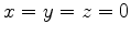 . The top row in Figure 4 shows the
back-projected vertical velocity
gradient and
gradient when source-receiver offset is zero. These back projections are often referred as
banana-donut kernels in the literature when transmission waves are under study (eg. Marquering et al. (1998); Rickett (2000); Marquering et al. (1999)).
Similar reflection tomography sensitivity kernel analysis for isotropic WEMVA operator can be found in Sava (2004) and Xie and Yang (2009).
. The top row in Figure 4 shows the
back-projected vertical velocity
gradient and
gradient when source-receiver offset is zero. These back projections are often referred as
banana-donut kernels in the literature when transmission waves are under study (eg. Marquering et al. (1998); Rickett (2000); Marquering et al. (1999)).
Similar reflection tomography sensitivity kernel analysis for isotropic WEMVA operator can be found in Sava (2004) and Xie and Yang (2009).
Compared with the
gradient, the
gradient has a nearly uniform strength with depth, while the
gradient fades away as
the wavepath moves away from the source and the receiver location. Also, the dominant energy of the
gradient points to the opposite direction
of the
gradient points. In fact, the
gradient is not reliable and should be ignored because
the wave that travels in the vertical direction is not sensitive to
.
When the source-receiver offset is
km, the gradients are shown in the middle row in Figure 4. Clearly, the back projections are spread along
the wavepaths from the source to the perturbed image point and from the perturbed image point to the receiver. In this case, the gradients in both
and
point in the same direction. Comparing the gradients in the cases of zero and nonzero offset, one can see that the vertical waves are more sensitive to
, and
the waves traveling at a large angle ( to the vertical in this case) are more sensitive to
. The bottom row in Figure 4
shows the summation of the gradients in these two cases, and confirms these observations.
to the vertical in this case) are more sensitive to
. The bottom row in Figure 4
shows the summation of the gradients in these two cases, and confirms these observations.
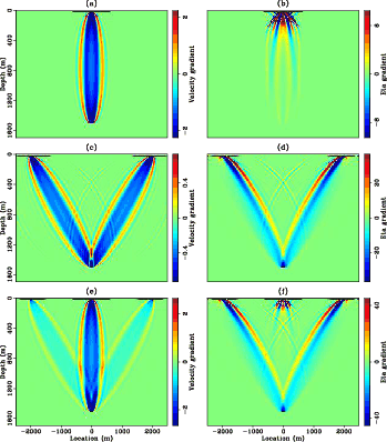
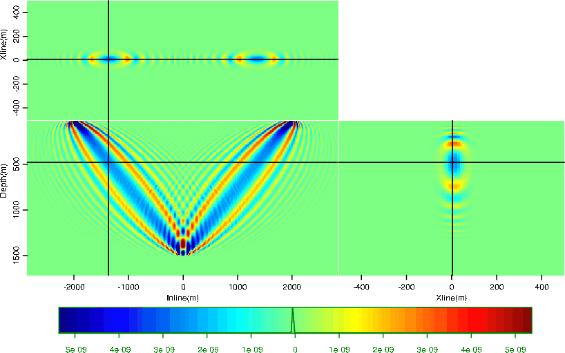
The 3D extension of this method is straightforward. The sensitivity kernels for
and
in 3D are shown in
Figures 5 and 6. A source and receiver pair with
km offset
are located at  . The 3D sensitivity kernels carry the same characteristics as the 2D kernels, only expanding to the crossline direction.
|
|---|
|
3dkernel-vel-new
Figure 5. 3D
kernel.
|
|
|
|
|---|
|
3dkernel-eta-new
Figure 6. 3D
kernel.
|
|
|
|
|
|
|
Wave-equation migration velocity analysis for VTI media using optimized implicit finite difference |