


Next: About this document ...
Up: Fomel & Biondi: t-x
Previous: AMO AMPLITUDE
amosym
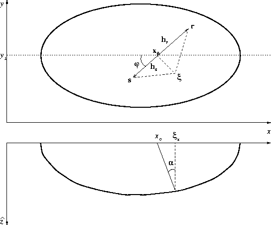
Figure 5 Reflection from the
ellipsoid of a prestack migration impulse response (a scheme). Top: Map view.
Bottom: Section of the ellipsoid with the plane drawn through the
central line and the reflection point.
|
|  |

This appendix describes the derivation of the main formulas for the
aperture evaluation that follow from the Fermat principle (18).
In order to avoid the algebraic
complications of (18), we simplify the
problem by taking into account the cylindrical symmetry of the ellipsoidal
reflector (15).
Consider a plane drawn through the reflection point and the central line
of the ellipsoid (the axis of the cylindrical symmetry). This plane
has to contain the central (normally reflected) ray from the
reflector. This conclusion follows from the fact that all the normal
reflections emerge at the central line because of the cylindrical
symmetry, as shown in Figure B-1. The intersection of the 3-D
reflector and the plane is the
2-D ellipse
|  |
(28) |
The connection between the emergence point of the normal ray x0 and
the x coordinate of the reflection point  can be derived from the
relationship evident in Figure B-1, as follows:
can be derived from the
relationship evident in Figure B-1, as follows:
|  |
(29) |
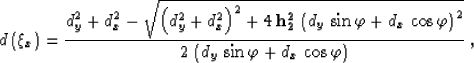
Equation (B-2) allows us to evaluate in terms of
x0 and get (19). The emergence point of the normal ray x0
corresponds to the
midpoint on an imaginary zero-offset section ( with a coincident
source and receiver). Therefore, the location of this point is
determined for given input
and output midpoints in accordance with expression (7).
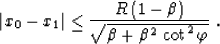
Obviously, the reflection point has to be inside the ellipse
(B-1). Therefore, its projection obeys the inequality
|  |
(30) |
As follows from (B-3), (B-2), and (16),
|  |
(31) |
Inequality (B-4) is the known aperture limitation of the DMO
operator (2) found by Deregowski and Rocca
1981. The equality in (B-4) is achieved
when the reflection point is on the surface, where the reflector dip
increases to 90 degrees.
Now the only unknown left in our problem is the y-coordinate of the
reflection point  . To find this unknown, we substitute
(19) into (17), choosing the convenient
parameterization
. To find this unknown, we substitute
(19) into (17), choosing the convenient
parameterization
|  |
(32) |
where 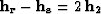 , and
, and 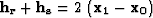 (Figure B-1). The
two-point traveltime function in (17) transforms to the form
(Figure B-1). The
two-point traveltime function in (17) transforms to the form
| 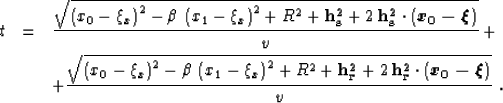 |
|
| (33) |
Applying the second equation from (18), we get a simple linear
equation for , which has the explicit solution (20).
From (19) and (20) one can find the reflection
point location for given midpoint and offset. To find the limits of
possible output midpoint locations, we constrain the reflection
point to be inside the ellipsoid (15) similarly to the way we did
in two dimensions when deriving (B-4). First, let's consider the
case of y2=y1 (the output midpoint  is on the line drawn
through
is on the line drawn
through  in the direction of the input azimuth). In this
case, combining expression (20) and inequality (21)
produces
in the direction of the input azimuth). In this
case, combining expression (20) and inequality (21)
produces
|  |
(34) |
For any azimuth rotation angle  less than 90 degrees, the
limitation (B-7) is smaller than that of the DMO operator
(B-4). The difference increases with the decrease of the
azimuth rotation, since the AMO aperture section
on the line y2=y1 monotonously shrinks to a point x2=x0=x1
when approaches zero. To extend this conclusion to the whole
3-D aperture, we can find the contour of the aperture by putting the
reflection point
at the edge of the ellipsoid (15), as follows:
less than 90 degrees, the
limitation (B-7) is smaller than that of the DMO operator
(B-4). The difference increases with the decrease of the
azimuth rotation, since the AMO aperture section
on the line y2=y1 monotonously shrinks to a point x2=x0=x1
when approaches zero. To extend this conclusion to the whole
3-D aperture, we can find the contour of the aperture by putting the
reflection point
at the edge of the ellipsoid (15), as follows:
|  |
(35) |
and solving (20) for y2. The aperture contour can then be defined by
the system of parametric expressions
|  |
(36) |
|  |
(37) |
where
|  |
(38) |
 ,and
,and 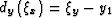 is defined by (B-8).
Next: About this document ...
Up: Fomel & Biondi: t-x
Previous: AMO AMPLITUDE
Stanford Exploration Project
9/12/2000