SHOT-GATHER BASED INTERPOLATION

Another possible application for using recursive steering filters is to interpolate seismic data. As an initial test we chose to interpolate a shot gather. We used a v(z) velocity function to construct hyperbolic trajectories, which in turn were used to construct our dip field (similar to the seismic dips used in the previous section).

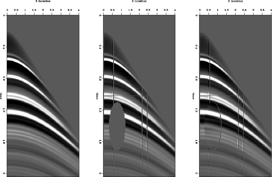
For a first test we created a synthetic shot gather using a v(z)=a+bz model as input to a finite difference code. We then cut a hole in this shot gather and attempted to recover the removed values. As Figure 8 shows we did a good job recovering the amplitude within a few iterations.

 

shot-s-combo
Figure 8 Left, synthetic shot gather; center, holes cut out of shot gather; right, inversion result after 15 iterations.

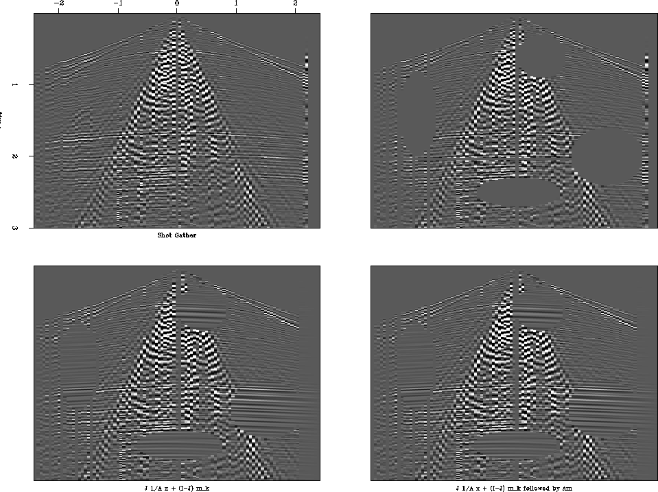
To see how the method reacted when it was given data that did not fit its model (in this case hyperbolic moveout) we used a dataset with significant noise problems (ground roll, bad traces, etc.). Using the same technique as in Figure 8 we ended up with a result which did a fairly decent job fitting portions of the data where noise content was low, but a poor job elsewhere (Figure 9). Even where the method did the best job of reconstructing the data, it still left a visible footprint. A more esthetically pleasing result can be achieved by using the above method followed a more traditional interpolation problem using the operator $\bold A$ and the fitting goal  

$$\bold A \bold m \approx 0 ,$$ (19)

where $\bold m$ is initialized with the result of our previous inversion problem and not allowed to change at locations where we have data. The bottom right panel in Figure 9 shows the result of applying a few iterations of fitting goal (19) to the bottom left result in Figure 9. By using both methodologies the interpolated data does a much better job blending into its surroundings but still is a poor interpolation result.

 

wz-25-combo
Figure 9 Top left, original shot gather; top right, gather with holes (input); bottom left, result applying equation 18, bottom right, result after applying equation (18) followed by (19).