WELL LOG/DIP INTERPOLATION

To illustrate the effectiveness of this method imagine a simple interpolation problem. Following the methodology of Fomel et al. (1997) we first bin the data, producing a model $\bold m$, composed of known data $\bold m_k$ and unknown data $\bold m_u$. We have an operator $\bold J$ which is simply a diagonal masking operator with zeros at known data locations and ones at unknown locations. We can write $\bold m_k$ and $\bold m_u$ in terms of $\bold m$ and $\bold J$,

$$\begin{eqnarray} \bold m_k &\approx& (\bold I\bold - \bold J)\bold m \ \bold m_u &\approx& \bold J \bold m\end{eqnarray}$$ (16) (17)

where $\bold{I}$ is the identity matrix. We have the preconditioning operator $\bold B$, which applies polynomial division using the helix methodology. In this case we have a single equation in our estimation problem,  

$$\bold m_k \approx (\bold I-\bold J) \bold B \bold x .$$ (18)

So the only question that remains is what to use for $\bold B$, or more specifically $\bold B^{-1}$, $\bold A$.

For this experiment we create a series of well logs by subsampling a 2-D velocity field. We use as our a priori information source, reflector dips, to build our steering filters, and thus our operator $\bold A$. For this test we pick our dips from our ``goal'', left portion of Figure 5. We define areas in which we believe each of these dips to be approximately correct, and smooth the overall field (right portion of Figure 5).

 

qdome-reflectors
Figure 5 Left, a synthetic seismic section with four picked reflectors indicated by '*'; right; the dip field constructed from the picked reflectors.

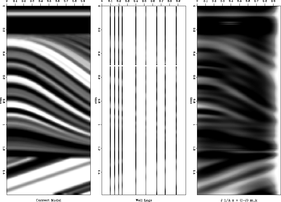
For the first test, we simulate nine well logs along the survey (Figure 6). We use equation (18) as our fitting goal and a conjugate gradient solver to estimate $\bold x$.Within 12 iterations we have a satisfactory solution(Figure 6). If you look closely, especially near the bottom of the section you can still see the well locations, but in general the solution converges quickly to something fairly close to the correct velocity field (Figure 5).

 

qdome-combo1
Figure 6 Left, correct velocity field; middle, well subset selected as input; right, velocity field resulting from interpolation.

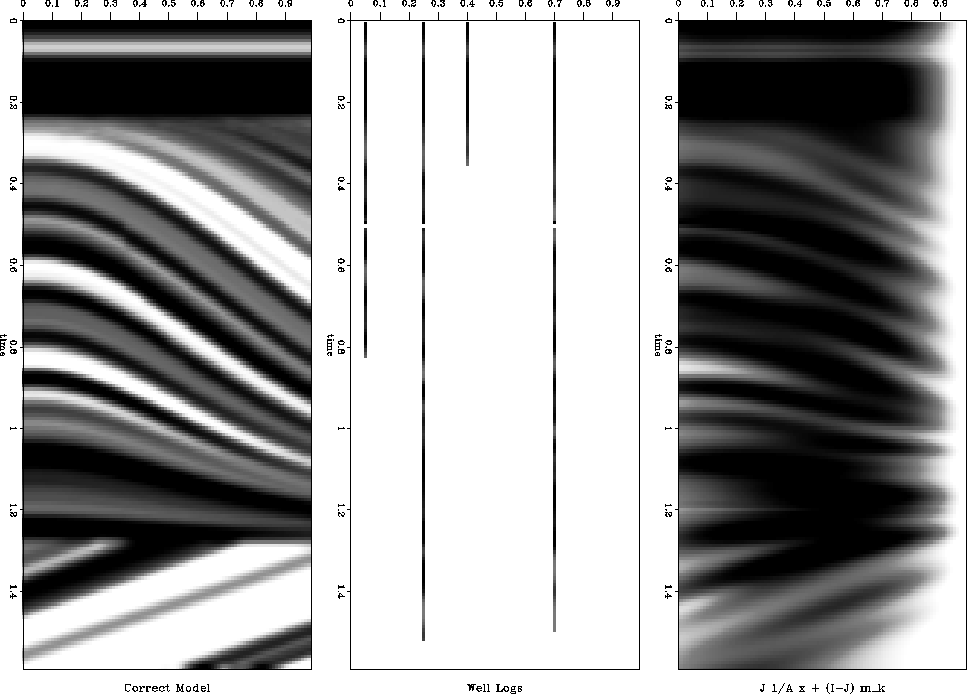
For a more difficult test, we decreased the number of wells, and give them varying lengths. In Figure 7 you see that in a few iterations we achieve a result quite similar to our goal. In addition, in areas far away from known data the method still followed the general dip direction simply at a lower frequency level.

 

qdome-combo4
Figure 7 Left model (our goal), middle well logs, and right estimated model after 12 iterations.