


Next: THE KINEMATICS OF OFFSET
Up: Fomel: Offset continuation
Previous: REFERENCES
To obtain an explicit solution of the Cauchy problem
(1)-(3), it is convenient to apply the following
simple transform of the function P:
|  |
(46) |
Here the Heavyside function H is included to take into account the
causality of the reflection seismic gathers (note that the time
tn=0 corresponds to the direct wave arrival). We can evenly
extrapolate the function Q to negative times, writing the reverse of
(47) as follows:
|  |
(47) |
With the change of function (47), equation (1)
transforms to
|  |
(48) |
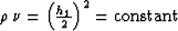
Applying the change of variables
|  |
(49) |
and Fourier transform in the midpoint coordinate y
|  |
(50) |
I further transform equation (49) to the canonical form of a
hyperbolic-type partial differential equation with two variables:
|  |
(51) |
The initial value conditions (2) and (3) in the
 space are defined on a hyperbola of the form
 . Now the solution
of the Cauchy problem follows directly from Riemann's method Courant (1962).
According to this method, the domain of dependence of each point
is a part of the hyperbola between the points
. Now the solution
of the Cauchy problem follows directly from Riemann's method Courant (1962).
According to this method, the domain of dependence of each point
is a part of the hyperbola between the points
 and
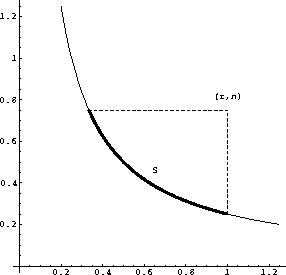
and  (Figure 4). If we let
  denote this curve, the solution takes an explicit integral form:
offrim
Figure 4
Domain of dependence of a point in the transformed coordinate system.
|
|  |


|  |
(52) |
Here R is the Riemann's function of equation (52), which has
the known explicit analytical expression
| 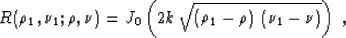 |
(53) |
where J0 is Bessel's function of zero order.
Integrating by parts and taking into account the connection of the
variables on the curve , we can simplify formula (55) to
the form
|  |
(54) |
where
| 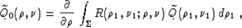 |
(55) |
| 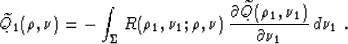 |
(56) |
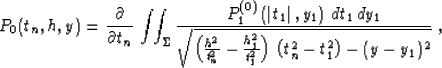
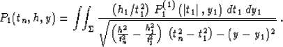
Applying the explicit expression for the Riemann's function R
(56) and performing the inverse transform of both the function and the
variables allows us to rewrite equations (57), (58), and
(59) in the original coordinate system. This yields the integral
offset continuation operators in the  domain
|  |
(57) |
where
|  |
(58) |
|  |
(59) |
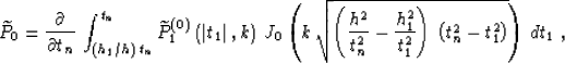
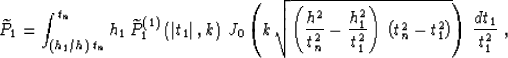
|  |
(60) |
|  |
(61) |
The inverse Fourier transforms of formulas (61) and (62) are
reduced to analytically evaluated integrals Gradshtein and Ryzhik (1994) to produce
explicit integral operators in the time-and-space domain
|  |
(62) |
where
|  |
(63) |
|  |
(64) |
The range of integration in (66) and (67) is
defined by inequality
|  |
(65) |
where  is in turn defined by formula (7). Formulas
(65), (66), and (67) coincide with (4),
(5), and (6) in the main text.
is in turn defined by formula (7). Formulas
(65), (66), and (67) coincide with (4),
(5), and (6) in the main text.
B
Next: THE KINEMATICS OF OFFSET
Up: Fomel: Offset continuation
Previous: REFERENCES
Stanford Exploration Project
4/19/2000