Examples

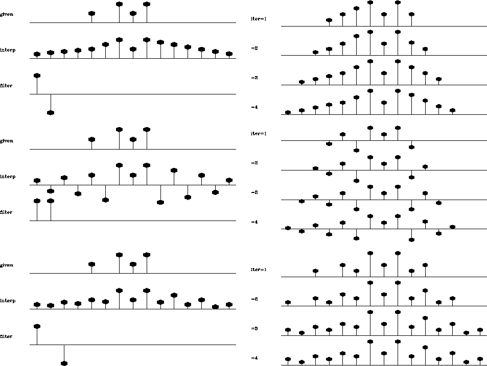
The first two examples in this paper are taken directly from Geophysical Exploration Mapping Claerbout (1997). They start from a simple 1-D synthetic data test. Figure 1 shows the interpolation results of the unpreconditioned technique with three different filters. For comparison with the preconditioned scheme, we changed the boundary convolution conditions from internal to truncated transient convolution. The system was solved with a conjugate-gradient iterative optimization.

 

mall
Figure 1 Unpreconditioned interpolation with three different regularization filters. On the left plot: the top shows the input data; the middle, the result of interpolation; and the bottom, the filter. The right plot shows the convergence process for the first four iterations.

As depicted on the right side of the figures, the interpolation process starts with a ``complicated'' model and slowly ``simplifies'' it until the final result is achieved.

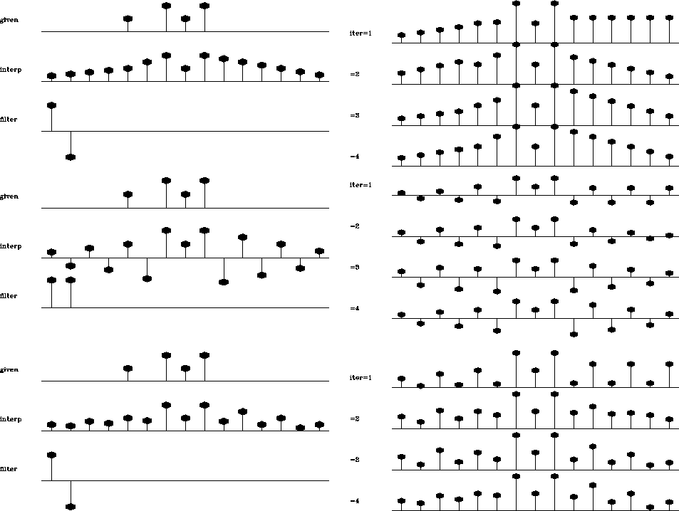
Preconditioned interpolation (Figure 2) behaves differently. At the early iterations, the model is simple. As the iteration proceeds, new details are added into the model. After a surprisingly small number of iterations, the output closely resembles the final output. This observation is fully consistent with the general theory of regularization and preconditioning Fomel (1997); Harlan (1995); Nichols (1994). The final output of interpolation with recursive deconvolution preconditioning is exactly the same as that of the original method.

 

sall
Figure 2 Interpolation with preconditioning. On the left plot: the top shows the input data; the middle, the result of interpolation; and the bottom, the filter. The right plot shows the convergence process for the first four iterations.

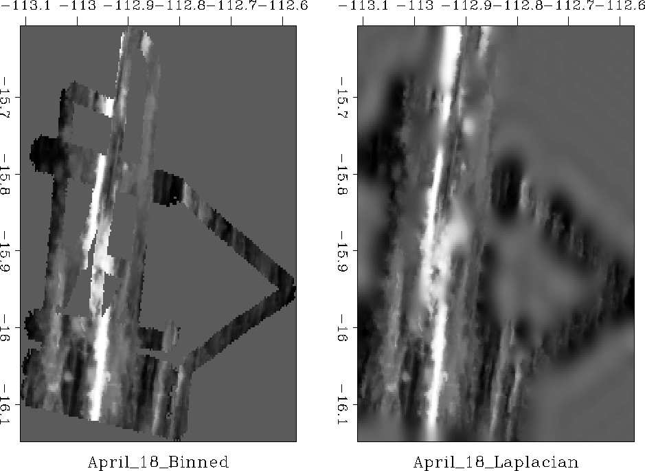
The next example is the SeaBeam dataset, a result of water bottom measurements from a single day of acquisition. This dataset has been used at SEP for benchmarking different strategies of data interpolation. The left plot in Figure 3 shows the original data. The right plot shows the result of (unpreconditioned) missing data interpolation with the Laplacian filter. The result is unsatisfactory, because the Laplacian filter doesn't absorb the spatial frequency distribution of the input dataset. We judge the quality of an interpolation scheme by its ability to hide the footprints of the acquisition geometry in the final result.

 

seabdat
Figure 3 On the left, the SeaBeam data: the depth of the ocean under ship tracks; on the right, an interpolation with the Laplacian filter.

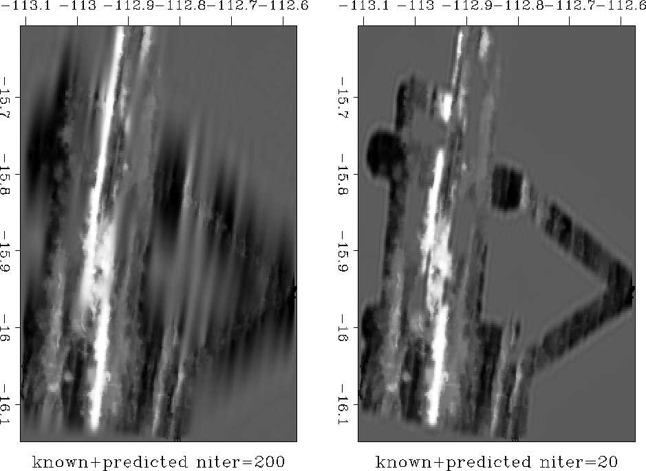
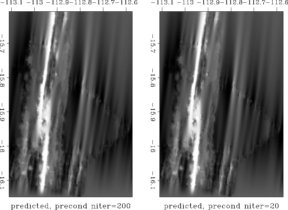
Claerbout (1997) obtains a significantly better result (Figure 4) by replacing the Laplacian filter with a prediction-error filter (PEF), estimated from the input data. The result in the left plot of Figure 4 was obtained after 200 conjugate-gradient iterations. If we stop after 20 iterations, the output (the right plot in Figure 4) shows only a small deviation from the input data. Large areas of the image remain unfilled.

 

seabold
Figure 4 SeaBeam interpolation with the prediction-error filter. The left plot was taken after 200 conjugate-gradient iterations; the right, after 20 iterations.

Inverting the PEF convolution with the help of the helix transform, we can now apply the inverse filtering operator to precondition the interpolation problem. As expected, the result after 200 iterations (the left plot in Figure 5) is similar to the result of the corresponding unpreconditioned interpolation. However, the output after just 20 iterations (the right plot in Figure 5) is already fairly close to the solution.

 

seabnew
Figure 5 SeaBeam interpolation with the inverse prediction-error filter. The left plot was taken after 200 conjugate-gradient iterations; the right, after 20 iterations.

For our third example we apply the preconditioning methodology to simulate interpolating well log velocities using reflector dip information as a guide. In the first two cases we used a space-invariant filter for our operator ${\bold D}$, and the corresponding inverse ${\bold P}$. In this example D is composed of a series of steering filters, small plane wave anihilators, oriented at some a priori angleClapp et al. (1997).

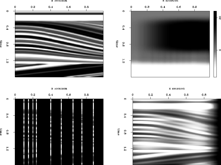
We started with a velocity field from a synthetic anticline model above a horizontal unconformity. To build the steering filters we make the assumption that velocity follows reflector dips. We first select four reflectors that characterize dip in the section (Figure qdome-combo1, top right). The selected dips are then interpolated to all model locations and smoothed (Figure qdome-combo1, top left). Using this dip field, the methodology in equation (6), and a series of well logs (Figure qdome-combo1, bottom left) constructed from the original velocity model, we attempted to reinterpolate the unknown velocities. The bottom right plot of Figure qdome-combo1 shows that the interpolation was successful in minimal iterations (in this case only 12 iterations were required).

 

qdome-combo1
Figure 6 Interpolating a synthetic velocity field from the well data. The left top plot shows the synthetic model; top right, the dip field for calculating steering filters; bottom left, the input data; bottom right, the interpolation result. Only 12 conjugate-gradient interpolations were required.