A SIMPLE derivation of the eikonal and transport equations

In this Appendix, I remind the reader how the eikonal equation is derived from the wave equation. The derivation is classic and can be found in many popular textbooks. See, for example, Cerveny et al. (1977).

Starting from the wave equation,  

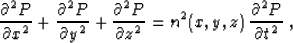$$\frac{\partial^2 P}{\partial x^2} + \frac{\partial^2 P}{\p... ...rtial z^2} = n^2 (x,y,z)\,\frac{\partial^2 P}{\partial t^2}\;,$$ (8)

we introduce a trial solution of the form  

$$P (x,y,t) = A (x,y,z) f (t - \tau (x,y,z))\;,$$ (9)

where $\tau$ is the eikonal, and A is the wave amplitude. The waveform function f is assumed to be a high frequency (discontinuous) signal. Substituting solution (9) into equation (8), we arrive at the constraint  

$$\Delta A \, f - 2 \nabla A \cdot \nabla \tau f' - A \Delta \tau f ' + A \left(\nabla \tau\right)^2 f'' = n^2 A f''\;.$$ (10)

Here $\Delta \equiv \nabla^2$ denotes the Laplacian operator. Equation (10) is as exact as the initial wave equation (8) and generally difficult to satisfy. However, we can try to satisfy it asymptotically, considering each of the high-frequency asymptotic components separately. The leading-order component corresponds to the second derivative of the wavelet f''. Isolating this component, we find that it is satisfied if and only if the traveltime function $\tau (x,y,z)$ satisfies the eikonal equation (1).

The next asymptotic order corresponds to the first derivative f'. It leads to the amplitude transport equation  

$$2 \nabla A \cdot \nabla \tau + A \Delta \tau = 0\;.$$ (11)

The amplitude, defined by equation (11), is often referred to as the amplitude of the zero-order term in the ray series. A series expansion of the function f in high-frequency asymptotic components produces recursive differential equations for the terms of higher order. In practice, equation (11) is sufficiently accurate for describing the major amplitude trends in most of the cases. It fails, however, in some special cases, such as caustics and diffraction.

B