Example 3: Leveled inverse interpolation

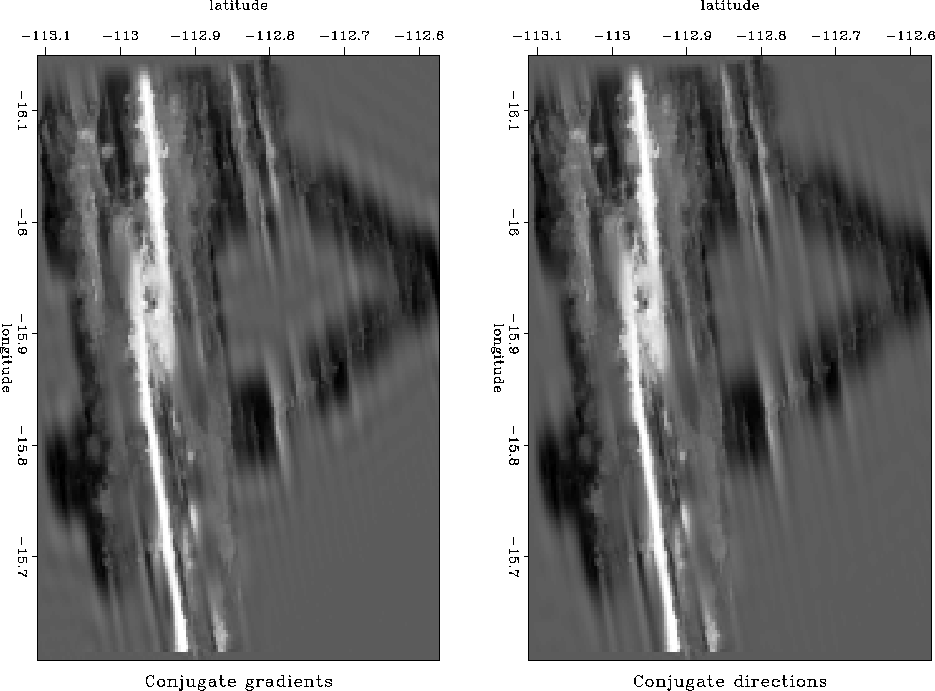
The third example is the linearized nonlinear inversion for interpolating the SeaBeam dataset Claerbout (1994); Crawley (1995b). This interpolation problem is nonlinear because the prediction-error filter is estimated simultaneously with the missing data. The conjugate-gradient solver showed a very slow convergence in this case. Figure 7 compares the results of the conjugate-gradient and conjugate-direction methods after 2500 iterations. Because of the large scale of the problem, I set niter=4 in the cdstep() program, storing only the three preceding steps of the conjugate-direction optimization. The acceleration of convergence produced a noticeably better interpolation, which is visible in the figure.

 

dirjbm
Figure 7 SeaBeam interpolation. Left plot: the result of the conjugate-gradient inversion after 2500 iterations. Right plot: the result of the short-memory conjugate-direction inversion after 2500 iterations.