

Next: Inverse Interpolation and Data
Up: Forward Interpolation
Previous: Beyond B-splines
For completeness, I conclude this section with two simple examples of
forward interpolation in seismic data processing.
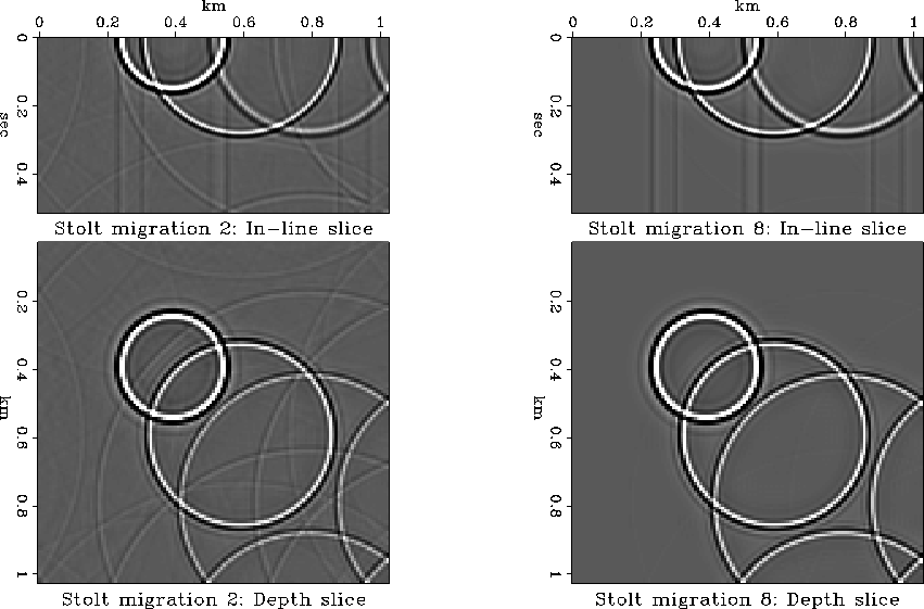
Figure ![[*]](http://sepwww.stanford.edu/latex2html/cross_ref_motif.gif) shows a 3-D impulse response of Stolt migration
Stolt (1978), computed by using 2-point linear
interpolation and 8-point B-spline interpolation. As noted by
Ronen (1982) and Harlan (1982),
inaccurate interpolation may lead to spurious artifact events in
Stolt-migrated image. Indeed, we see several artifacts for the image
with linear interpolation (the left plots in Figure
shows a 3-D impulse response of Stolt migration
Stolt (1978), computed by using 2-point linear
interpolation and 8-point B-spline interpolation. As noted by
Ronen (1982) and Harlan (1982),
inaccurate interpolation may lead to spurious artifact events in
Stolt-migrated image. Indeed, we see several artifacts for the image
with linear interpolation (the left plots in Figure ![[*]](http://sepwww.stanford.edu/latex2html/cross_ref_motif.gif) .)
The artifacts are removed by a more accurate interpolation method (the
right plots in Figure
.)
The artifacts are removed by a more accurate interpolation method (the
right plots in Figure ![[*]](http://sepwww.stanford.edu/latex2html/cross_ref_motif.gif) .)
stolt
.)
stolt
Figure 25 Stolt migration impulse response. Left: using
linear interpolation. Right: using seventh-order B-spline
interpolation. Migration artifacts are removed by a more accurate
forward interpolation method.


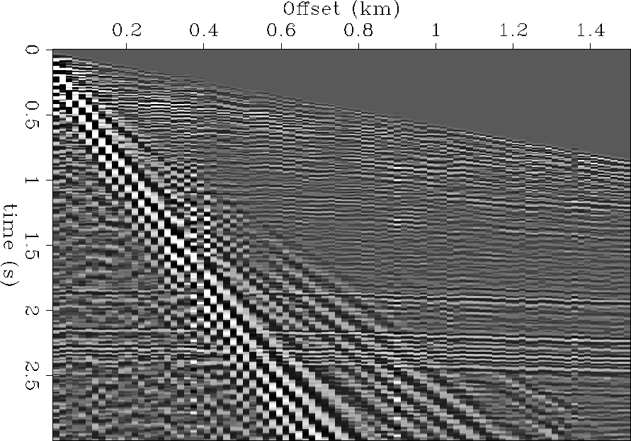
Another simple example is radial trace transform
Ottolini (1982) Figure ![[*]](http://sepwww.stanford.edu/latex2html/cross_ref_motif.gif) shows a land shot
gather contaminated by nearly radial ground-roll. As discussed by
Claerbout (1983), Henley (1999), and
Brown and Claerbout (2000), one can effectively eliminate
ground-roll noise by applying radial trace transform, followed by
high-pass filtering and the inverse radial transform.
Figure
shows a land shot
gather contaminated by nearly radial ground-roll. As discussed by
Claerbout (1983), Henley (1999), and
Brown and Claerbout (2000), one can effectively eliminate
ground-roll noise by applying radial trace transform, followed by
high-pass filtering and the inverse radial transform.
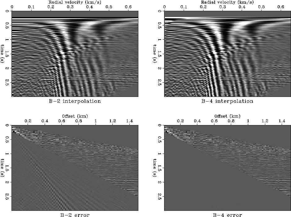
Figure ![[*]](http://sepwww.stanford.edu/latex2html/cross_ref_motif.gif) shows the result of the forward radial
transform of the shot gather in Figure
shows the result of the forward radial
transform of the shot gather in Figure ![[*]](http://sepwww.stanford.edu/latex2html/cross_ref_motif.gif) in the
radial band of the ground-roll noise and the transform error after
going back to the original domain. Comparing the results of using
linear and third-order B-spline interpolation, we see once again that
the transform artifacts are removed with a more accurate interpolation
scheme.
in the
radial band of the ground-roll noise and the transform error after
going back to the original domain. Comparing the results of using
linear and third-order B-spline interpolation, we see once again that
the transform artifacts are removed with a more accurate interpolation
scheme.
radialdat
Figure 26 Ground-roll-contaminated shot
gather used in a radial transform test
|
|  |


 radial
Figure 27 Radial trace transform results. Top: radial
trace domain. Bottom: residual error after the inverse transform.
The error should be zero in a radial band from 0 to 0.65 km/s radial
velocity. Left: using linear interpolation. Right: using third-order
B-spline interpolation.


Next: Inverse Interpolation and Data
Up: Forward Interpolation
Previous: Beyond B-splines
Stanford Exploration Project
11/9/2000
![[*]](http://sepwww.stanford.edu/latex2html/cross_ref_motif.gif) shows a 3-D impulse response of Stolt migration
Stolt (1978), computed by using 2-point linear
interpolation and 8-point B-spline interpolation. As noted by
Ronen (1982) and Harlan (1982),
inaccurate interpolation may lead to spurious artifact events in
Stolt-migrated image. Indeed, we see several artifacts for the image
with linear interpolation (the left plots in Figure
shows a 3-D impulse response of Stolt migration
Stolt (1978), computed by using 2-point linear
interpolation and 8-point B-spline interpolation. As noted by
Ronen (1982) and Harlan (1982),
inaccurate interpolation may lead to spurious artifact events in
Stolt-migrated image. Indeed, we see several artifacts for the image
with linear interpolation (the left plots in Figure ![[*]](http://sepwww.stanford.edu/latex2html/cross_ref_motif.gif) .)
The artifacts are removed by a more accurate interpolation method (the
right plots in Figure
.)
The artifacts are removed by a more accurate interpolation method (the
right plots in Figure ![[*]](http://sepwww.stanford.edu/latex2html/cross_ref_motif.gif) .)
.)

![[*]](http://sepwww.stanford.edu/latex2html/cross_ref_motif.gif) shows a land shot
gather contaminated by nearly radial ground-roll. As discussed by
Claerbout (1983), Henley (1999), and
Brown and Claerbout (2000), one can effectively eliminate
ground-roll noise by applying radial trace transform, followed by
high-pass filtering and the inverse radial transform.
Figure
shows a land shot
gather contaminated by nearly radial ground-roll. As discussed by
Claerbout (1983), Henley (1999), and
Brown and Claerbout (2000), one can effectively eliminate
ground-roll noise by applying radial trace transform, followed by
high-pass filtering and the inverse radial transform.
Figure ![[*]](http://sepwww.stanford.edu/latex2html/cross_ref_motif.gif) shows the result of the forward radial
transform of the shot gather in Figure
shows the result of the forward radial
transform of the shot gather in Figure ![[*]](http://sepwww.stanford.edu/latex2html/cross_ref_motif.gif) in the
radial band of the ground-roll noise and the transform error after
going back to the original domain. Comparing the results of using
linear and third-order B-spline interpolation, we see once again that
the transform artifacts are removed with a more accurate interpolation
scheme.
in the
radial band of the ground-roll noise and the transform error after
going back to the original domain. Comparing the results of using
linear and third-order B-spline interpolation, we see once again that
the transform artifacts are removed with a more accurate interpolation
scheme.
