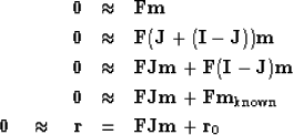
For the operator approach to the fitting goal
![]() we rewrite it as
we rewrite it as
![]() where
where
![\begin{displaymath}
-\bold F_k \bold m_k
\quad \approx \quad
\left[
\begin{arra...
...
m_6
\end{array} \right]
\quad =\quad \bold F \bold J \bold m\end{displaymath}](img26.gif) |
(3) |
 |
(4) | |
| (5) | ||
| (6) | ||
| (7) | ||
| (8) |
| |
(9) |
We begin the calculation with
the known data values where missing data values are replaced by zeros, namely
![]() .Filter this data,
getting
.Filter this data,
getting ![]() ,and load it into the residual
,and load it into the residual ![]() .With this initialization completed,
we begin an iteration loop.
First we compute
.With this initialization completed,
we begin an iteration loop.
First we compute ![]() from equation (9).
from equation (9).
| (10) |
| |
(11) |
I could have passed a new operator ![]() into the old solver,
but found it worthwhile to write a new,
more powerful solver having built-in constraints.
To introduce the masking operator
into the old solver,
but found it worthwhile to write a new,
more powerful solver having built-in constraints.
To introduce the masking operator ![]() into the solver_smp
subroutine
into the solver_smp
subroutine ![[*]](http://sepwww.stanford.edu/latex2html/cross_ref_motif.gif) ,
I introduce an optional operator Jop,
which is initialized with a logical array of the model size.
Two lines in the solver_tiny module
,
I introduce an optional operator Jop,
which is initialized with a logical array of the model size.
Two lines in the solver_tiny module ![[*]](http://sepwww.stanford.edu/latex2html/cross_ref_motif.gif)
stat = Fop( T, F, g, rd)                          #  g = F' Rd
stat = Fop( F, F, g, gd)                          #  G = F  g
become three lines in the standard library module solver_smp.
(We use a temporary array tm of the size of model space.)
![]() is g and
is g and
![]() is gg.
is gg.
stat = Fop( T, F, g, rd)                                  # g = F' Rd
if ( present( Jop)) { tm=g;  stat= Jop( F, F, tm, g)      # g = J g
stat = Fop( F, F, g, gg)                                  # G = F g
The full code includes all the definitions we had earlier
in solver_tiny module ![[*]](http://sepwww.stanford.edu/latex2html/cross_ref_motif.gif) .
Merging it with the above bits of code we have
the simple solver solver_smp.
solver_smpsimple solver
.
Merging it with the above bits of code we have
the simple solver solver_smp.
solver_smpsimple solver
There are two methods of invoking the solver. Comment cards in the code indicate the slightly more verbose method of solution which matches the theory presented in the book.
The subroutine to find missing data is mis1().
It assumes that zero values in the input data
correspond to missing data locations.
It uses our convolution operator
tcai1() ![[*]](http://sepwww.stanford.edu/latex2html/cross_ref_motif.gif) .
You can also check the Index for other
operators and modules.
mis11-D missing data
.
You can also check the Index for other
operators and modules.
mis11-D missing data
I sought reference material on conjugate gradients with constraints
and didn't find anything,
leaving me to fear that this chapter was in error
and that I had lost the magic property of convergence
in a finite number of iterations.
I tested the code and it did converge in a finite number of iterations.
The explanation is that these constraints are almost trivial.
We pretended we had extra variables,
and computed a ![]() for each of them.
Then we set the
for each of them.
Then we set the ![]() to zero,
hence making no changes to anything,
like as if we had never calculated the extra
to zero,
hence making no changes to anything,
like as if we had never calculated the extra ![]() 's.
's.
