 |
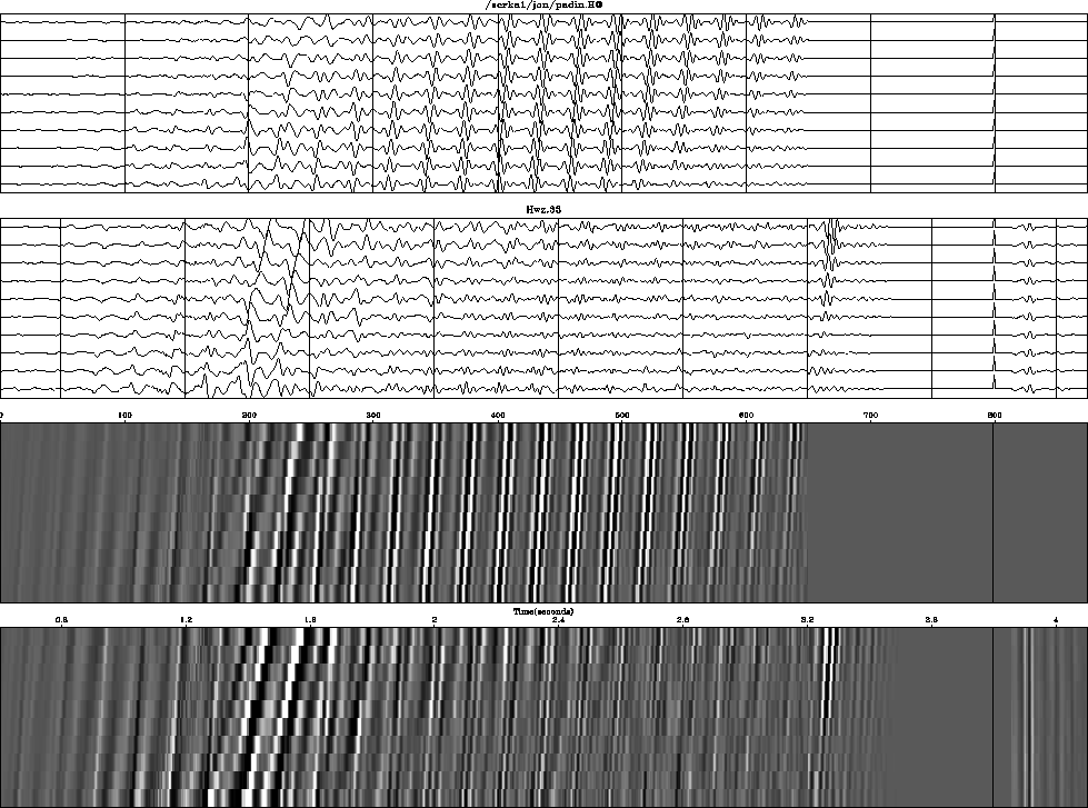
Figure 12 Data from the North Sea (extracted from Yilmaz and Cumro dataset 33) processed by prediction error. Rightmost box is weighted according to the desired stabilization. The truncation event is weighted by zero.
![[*]](http://sepwww.stanford.edu/latex2html/cross_ref_motif.gif) ) and
(
) and
(![[*]](http://sepwww.stanford.edu/latex2html/cross_ref_motif.gif) ),
was described earlier in this book.
I installed this stabilization, along with the filter determinations
discussed in this chapter,
but as I expected,
stabilization in this highly overdetermined application
showed no advantages.
Nevertheless, it is worth seeing how stabilization is implemented,
particularly since the changes to the program
calling iner()
make for more informative plots.
),
was described earlier in this book.
I installed this stabilization, along with the filter determinations
discussed in this chapter,
but as I expected,
stabilization in this highly overdetermined application
showed no advantages.
Nevertheless, it is worth seeing how stabilization is implemented,
particularly since the changes to the program
calling iner()
make for more informative plots.
The input data is modified by appending a zero-padded impulse at the data's end. The output will contain the filter impulse response in that region. The spike size is chosen to be compatible with the data size, for the convenience of the plotting programs. The weighting function in the appended region is scaled according to how much stabilization is desired. Figure 12 shows the complete input and residual.
 |
It also illustrates the problem that output data flows beyond the length of the input data because of the nonzero length of the filter. This extra output is undoubtedly affected by the truncation of the data, and its energy should not be part of the energy minimization. Therefore it is weighted by zero.
![[*]](http://sepwww.stanford.edu/latex2html/cross_ref_motif.gif) .
(Notice that the coefficients depend on
.
(Notice that the coefficients depend on ![[*]](http://sepwww.stanford.edu/latex2html/cross_ref_motif.gif) .
.