Next: Two-layer model
Up: SLANT STACK
Previous: Slant stacking and linear
A slant stack of a data gather yields a single trace
characterized by the slant parameter p.
Slant stacking at many p-values yields a
slant-stack gather. (Those with a strong mathematical-physics background
will note that slant stacking transforms travel-time curves
by the Legendre transformation.
Especially clear background reading is found in
Thermodynamics,
by H.B. Callen, Wiley, 1960, pp. 90-95).
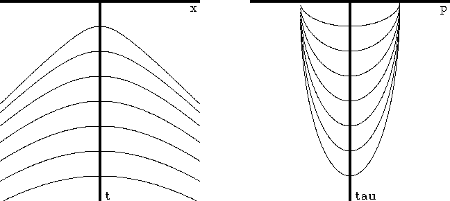
Let us see what happens to the familiar family of hyperbolas
t2 v2 = zj2 + x2 when we slant stack.
It will be convenient to consider the circle and hyperbola
equations in parametric form,
that is,
instead of t2 v2 = x2 + z2,
we use  and
and  or
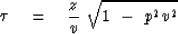
or  .Take the equation for linear moveout
|  |
(9) |
and eliminate t and x with the parametric equations.
|  |
(10) |
|  |
(11) |
Squaring gives the familiar ellipse equation
| 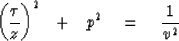 |
(12) |
Equation (12) is plotted in Figure 6
for various reflector depths zj.
sstt
Figure 6
Travel-time curves for a data gather on a multilayer earth model of
constant velocity before and after slant stacking.


Next: Two-layer model
Up: SLANT STACK
Previous: Slant stacking and linear
Stanford Exploration Project
10/31/1997