From the assumption that experimental data
can be fit to hyperbolas
(each with a different velocity and each with a different apex ![]() )let us next see how
we can fit an earth model of layers,
each with a constant velocity.
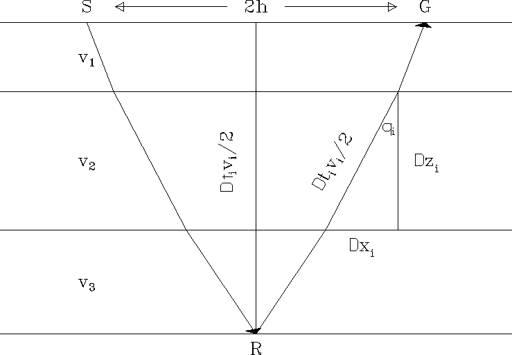
Consider the horizontal reflector
overlain by a stratified interval velocity v(z)
shown in Figure 10.
)let us next see how
we can fit an earth model of layers,
each with a constant velocity.
Consider the horizontal reflector
overlain by a stratified interval velocity v(z)
shown in Figure 10.
|
stratrms
Figure 10 Raypath diagram for normal moveout in a stratified earth. |  |
The separation between the source and geophone,
also called the offset, is 2h and the total travel time is t.
Travel times are not be precisely hyperbolic,
but it is common practice to find the best fitting hyperbolas,
thus finding the function ![]() .
.
| |
(24) |
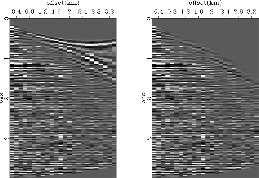
An example of using equation (24)
to stretch t into ![]() is shown in Figure 11.
(The programs that
find the required
is shown in Figure 11.
(The programs that
find the required ![]() and do the stretching are coming up in
chapter
and do the stretching are coming up in
chapter ![[*]](http://sepwww.stanford.edu/latex2html/cross_ref_motif.gif) .)
.)
 |
Equation (21) shows that
![]() is
the ``root-mean-square'' or
``RMS'' velocity defined by
an average of v2 over the layers.
Expressing it for a small number of layers we get
is
the ``root-mean-square'' or
``RMS'' velocity defined by
an average of v2 over the layers.
Expressing it for a small number of layers we get
| |
(25) |
| |
(26) |
| |
(27) |
Next we examine an important practical calculation,
getting interval velocities from measured RMS velocities:
Define
in layer i,
the interval velocity vi
and the two-way vertical travel time ![]() .Define the RMS velocity
of a reflection
from the bottom of the i-th layer
to be Vi.
Equation (25) tells us that for
reflections from the bottom of the first, second, and third layers we have
.Define the RMS velocity
of a reflection
from the bottom of the i-th layer
to be Vi.
Equation (25) tells us that for
reflections from the bottom of the first, second, and third layers we have
 |
(28) | |
| (29) | ||
| (30) |
Normally it is easy to measure the times of the three hyperbola tops,
![]() ,
,
![]() and
and
![]() .Using methods in chapter
.Using methods in chapter ![[*]](http://sepwww.stanford.edu/latex2html/cross_ref_motif.gif) we can measure the RMS velocities V2 and V3.
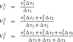
With these we can solve for the interval velocity v3 in the third layer.
Rearrange (30) and (29) to get
we can measure the RMS velocities V2 and V3.
With these we can solve for the interval velocity v3 in the third layer.
Rearrange (30) and (29) to get
| |
(31) | |
| (32) |
| |
(33) |