Kirchhoff versus phase-shift migration

In chapter , we were introduced to the Kirchhoff migration and modeling method by means of subroutines kirchslow() and kirchfast() . From chapter  we know that these routines should be supplemented by a $\sqrt{-i\omega}$filter such as subroutine halfdifa() . Here, however, we will compare results of the unadorned subroutine kirchfast() with our new programs, phasemig() and phasemod() . Figure 7 shows the result of modeling data and then migrating it. Kirchhoff and phase-shift migration methods both work well. As expected, the Kirchhoff method lacks some of the higher frequencies that could be restored by $\sqrt{-i\omega}$.Another problem is the irregularity of the shallow bedding. This is an operator aliasing problem addressed in chapter .

 

comrecon
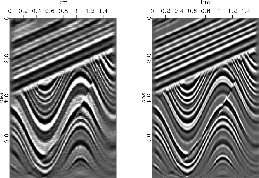
Figure 7 Reconstruction after modeling. Left is by the nearest-neighbor Kirchhoff method. Right is by the phase shift method.

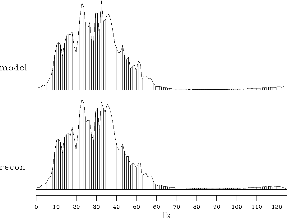
Figure 8 shows the temporal spectrum of the original sigmoid model, along with the spectrum of the reconstruction via phase-shift methods. We see the spectra are essentially identical with little growth of high frequencies as we noticed with the Kirchhoff method in Figure .

 

phaspec Figure 8 Top is the temporal spectrum of the model. Bottom is the spectrum of the reconstructed model.

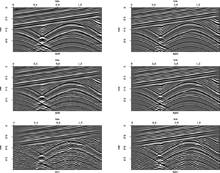
Figure 9 shows the effect of coarsening the space axis. Synthetic data is generated from an increasingly subsampled model. Again we notice that the phase-shift method of this chapter produces more plausible results than the simple Kirchhoff programs of chapter .

 

commod
Figure 9 Modeling with increasing amounts of lateral subsampling. Left is the nearest-neighbor Kirchhoff method. Right is the phase-shift method. Top has 200 channels, middle has 100 channels, and bottom has 50 channels.