![[*]](http://sepwww.stanford.edu/latex2html/cross_ref_motif.gif) .
.
Triangle smoothing
is rectangle smoothing done twice.
For a mathematical description of the triangle filter,
we simply square equation (10).
Convolving a rectangle function with itself many times yields
a result that mathematically tends towards a Gaussian function.
Despite the sharp corner on the top of the triangle function,
it has a shape that is remarkably similar to a Gaussian,
as we can see by looking at
Figure ![[*]](http://sepwww.stanford.edu/latex2html/cross_ref_motif.gif) .
.
With filtering, end effects can be a nuisance.
Filtering increases the length of the data,
but people generally want to keep input and output
the same length (for various practical reasons).
This is particularly true when filtering a space axis.
Suppose the five-point signal (1, 1,1,1,1)
is smoothed using the boxconv() program
with the three-point smoothing filter (1,1,1)/3.
The output is 5+3-1 points long, namely,
(1,2,3,3,3,2,1)/3.
We could simply abandon the points off the ends,
but I like to fold them back in,
getting instead (1+2,3,3,3,1+2).
An advantage of the folding is that a constant-valued signal
is unchanged by the smoothing.
This is desirable since a smoothing filter is a low-pass filter
which naturally should pass the lowest frequency ![]() without distortion.
The result is like a wave reflected by a
zero-slope
end condition.
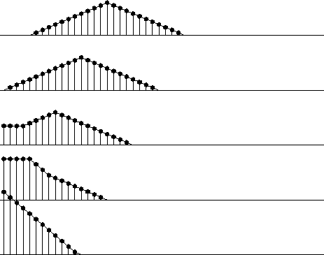
Impulses are smoothed into triangles except near the boundaries.
What happens near the boundaries is shown in Figure 3.
without distortion.
The result is like a wave reflected by a
zero-slope
end condition.
Impulses are smoothed into triangles except near the boundaries.
What happens near the boundaries is shown in Figure 3.
|
triend
Figure 3 Edge effects when smoothing an impulse with a triangle function. Inputs are spikes at various distances from the edge. |  |
Note that at the boundary, there is necessarily only half a triangle, but it is twice as tall.
Figure 3 was derived from the routine triangle().
# Convolve with triangle
#
subroutine triangle( nr, m1, n12, uu, vv)
# input:        nr      rectangle width (points) (Triangle base twice as wide.)
# input:        uu(m1,i2),i2=1,n12      is a vector of data.
# output:       vv(m1,i2),i2=1,n12      may be on top of uu
integer nr,m1,n12, i,np,nq
real uu( m1, n12),  vv( m1, n12)
temporary real pp(n12+nr-1), qq(n12+nr+nr-2), tt(n12)
do i=1,n12 {    qq(i) = uu(1,i) }
if( n12 == 1 )
        call copy( n12, qq, tt)
else {
        call boxconv( nr, n12, qq, pp);         np = nr+n12-1
        call boxconv( nr, np , pp, qq);         nq = nr+np-1
        do i= 1, n12
                        tt(i) = qq(i+nr-1)
        do i= 1, nr-1                                   # fold back near end
                        tt(i) = tt(i) + qq(nr-i)
        do i= 1, nr-1                                   # fold back far end
                        tt(n12-i+1) = tt(n12-i+1) + qq(n12+(nr-1)+i)
        }
do i=1,n12 {    vv(1,i) = tt(i) }
return; end
I frequently use this program, so it is cluttered with extra features.
For example, the output can share the same location as the input.
Further, since it is commonly necessary to smooth along the 2-axis
of a two-dimensional array,
there are some Fortran-style pointer manipulations to allow
the user to smooth either the 1-axis or the 2-axis.
For those of you unfamiliar with Fortran matrix-handling tricks,
I include below another routine, triangle2(), that teaches how
a two-dimensional array can be smoothed over both its 1-axis
and its 2-axis.
Some examples of two-dimensional smoothing are given in chapter ![[*]](http://sepwww.stanford.edu/latex2html/cross_ref_motif.gif) .
.
# smooth by convolving with triangle in two dimensions.
#
subroutine triangle2( rect1, rect2, n1, n2, uu, vv)
integer i1,i2,        rect1, rect2, n1, n2
real uu(n1,n2), vv(n1,n2)
temporary real ss(n1,n2)
do i1= 1, n1
                call triangle( rect2, n1, n2, uu(i1,1), ss(i1,1))
do i2= 1, n2
                call triangle( rect1,  1, n1, ss(1,i2), vv(1,i2))
return; end
![[*]](http://sepwww.stanford.edu/latex2html/cross_ref_motif.gif) .
1
.
1