Variance of the sample mean

Our objective here is to calculate how far the estimated mean $\hat m$ is likely to be from the true mean m for a sample of length n. This difference is the variance of the sample mean and is given by $(\Lambda m)^2=\sigma_{\hat m}^2$, where

$$\begin{eqnarray} \sigma_{\hat m}^2 &= & \E\, [(\hat{m} - m)^2] \ &= & \E\, \left\{ [(\sum w_t x_t) - m]^2 \right\}\end{eqnarray}$$ (23) (24)

Now use the fact that $m = m\sum w_t = \sum w_t m$:

$$\begin{eqnarray} \sigma_{\hat m}^2 &= &\E\, \left\{ \left[\sum_t w_t (x_t - m) ... ...\ &= &\E\, \left[\sum_t \sum_s w_t w_s (x_t - m)(x_s - m) \right] \end{eqnarray}$$ (25) (26) (27)

The step from (26) to (27) follows because

$$(a_1+a_2+a_3)\, (a_1+a_2+a_3) \eq {\rm sum \; of} \quad \lef... ... & a_2 a_3 \ a_3 a_1 & a_3 a_2 & a_3 a_3 \end{array}\right]$$ (28)

The expectation symbol $\E$ can be regarded as another summation, which can be done after, as well as before, the sums on t and s, so  

$$\sigma_{\hat m}^2 \eq \sum_t \sum_s w_t \, w_s\, \E\, \left[ (x_t - m)(x_s - m) \right]$$ (29)

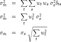
If $t\neq s$, since x_t and x_s are independent of each other, the expectation $\E[(x_t - m)(x_s - m)]$ will vanish. If s = t, then the expectation is the variance defined by (13). Expressing the result in terms of the Kronecker delta, $\delta_{ts}$(which equals unity if t=s, and vanishes otherwise) gives

$$\begin{eqnarray} \sigma_{\hat m}^2 &= & \sum_t \sum_s w_t \, w_s \, \sigma_x^2... ...ma_x^2 \ \sigma_{\hat m} &= & \sigma_x \ \sqrt{ \sum_t w^2_t }\end{eqnarray}$$ (30) (31) (32)

For n weights, each of size 1/n, the standard deviation of the sample mean is  

$$\Lambda m_x \eq \sigma_{\hat m_x} \eq \sigma_x \ \sqrt{ \su... ...\left( {1 \over n}\right)^2 } \eq {\sigma_x \over \sqrt{n} }$$ (33)

This is the most important property of random numbers that is not intuitively obvious. Informally, the result (33) says this: given a sum y of terms with random polarity, whose theoretical mean is zero, then

$$y \eq \underbrace{\pm 1 \pm 1 \pm 1 \cdots}_{n\ {\rm terms}}$$ (34)

The sum y is a random variable whose standard deviation is $\sigma_y=\sqrt{n}=\Lambda y$.An experimenter who does not know the mean is zero will report that the mean of y is $\E (y) = \hat y \pm \Lambda y$,where $\hat y$ is the experimental value.

If we are trying to estimate the mean of a random series that has a time-variable mean, then we face a basic dilemma. Including many numbers in the sum in order to make $\Lambda m$ small conflicts with the possibility of seeing m_t change during the measurement.

The ``variance of the sample variance'' arises in many contexts. Suppose we want to measure the storminess of the ocean. We measure water level as a function of time and subtract the mean. The storminess is the variance about the mean. We measure the storminess in one minute and call it a sample storminess. We compare it to other minutes and other locations and we find that they are not all the same. To characterize these differences, we need the variance of the sample variance $\sigma_{\hat \sigma^2}^2$.

Some of these quantities can be computed theoretically, but the computations become very cluttered and dependent on assumptions that may not be valid in practice, such as that the random variables are independently drawn and that they have a Gaussian probability function. Since we have such powerful computers, we might be better off ignoring the theory and remembering the basic principle that a function of random numbers is also a random number. We can use simulation to estimate the function's mean and variance.

Basically we are always faced with the same dilemma: if we want to have an accurate estimation of the variance, we need a large number of samples, which limits the possibility of measuring a time-varying variance.

EXERCISES:

1. Suppose the mean of a sample of random numbers is estimated by a triangle weighting function, i.e.,

   $$\hat{m} \eq s \sum^n_{i = 0} (n - i)\, x_i$$

   Find the scale factor s so that $\E(\hat{m}) = m$.Calculate $\Lambda m$.Define a reasonable $\Lambda T$.Examine the uncertainty relation.
2. A random series x_t with a possibly time-variable mean may have the mean estimated by the feedback equation

   $$\hat{m}_t \eq (1 - \epsilon) \hat{m}_{t-1} + b x_t$$

   a.

   Express $\hat{m}_t$ as a function of $x_t, x_{t-1}, \ldots ,$and not $\hat{m}_{t - 1}$.

   b.

   What is $\Lambda T$, the effective averaging time?

   c.

   Find the scale factor b so that if m_t = m, then $\E(\hat{m}_t) = m.$

   d.

   Compute the random error $\Lambda m = \sqrt{\E(\hat{m} - m)^2 }$.(HINT: $\Lambda m$ goes to $\sigma \sqrt{\epsilon/2 }$ as $\epsilon \rightarrow 0$.)

   e.

   What is $(\Lambda m)^2 \Lambda T$ in this case?