2-D INTERPOLATION BEYOND ALIASING

 I have long marveled at the ability of humans to interpolate seismic data containing mixtures of dips where spatial frequencies exceed the Nyquist limits. These limits are hard limits on migration programs. Costly field-data-acquisition activities are designed with these limits in mind. I feared this human skill of going beyond the limit was deeply nonlinear and beyond reliable programming. Now, however, I have obtained results comparable in quality to those of S. Spitz, and I am doing so in a way that seems reliable--using two-stage, linear least squares. First we will look at some results and then examine the procedure. Before this program can be applied to field data for migration, remember that the data must be broken into many overlapping tiles of about the size shown here and the results from each tile pieced together.

 

lace3
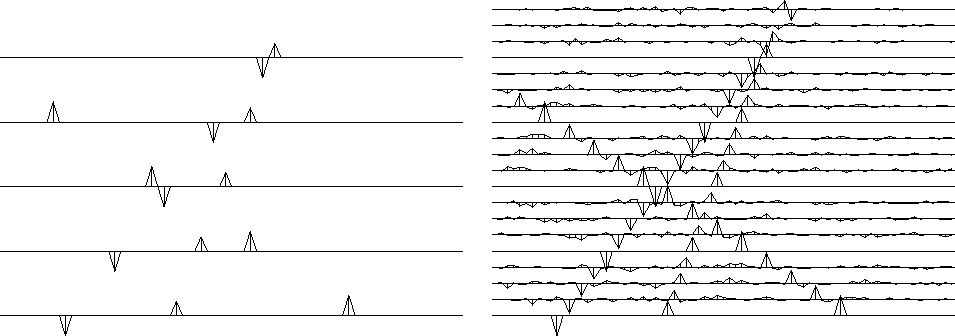
Figure 13 Left is five signals, each showing three arrivals. Using the data shown on the left (and no more), the signals have been interpolated. Three new traces appear between each given trace as shown on the right.

Figure 13 shows three plane waves recorded on five channels and the interpolated data. Both the original data and the interpolated data can be described as ``beyond aliasing'' because on the input data the signal shifts exceed the signal duration. The calculation requires only a few seconds of a ``two-stage least-squares'' method, where the first stage estimates an inverse covariance matrix of the known data, and the second uses it to estimate the missing traces. Actually, a 2-D prediction-error filter

is estimated, and the inverse covariance matrix, which amounts to the PE filter times its adjoint, is not needed explicitly.

 

lace2
Figure 14 Two plane waves and their interpolation.

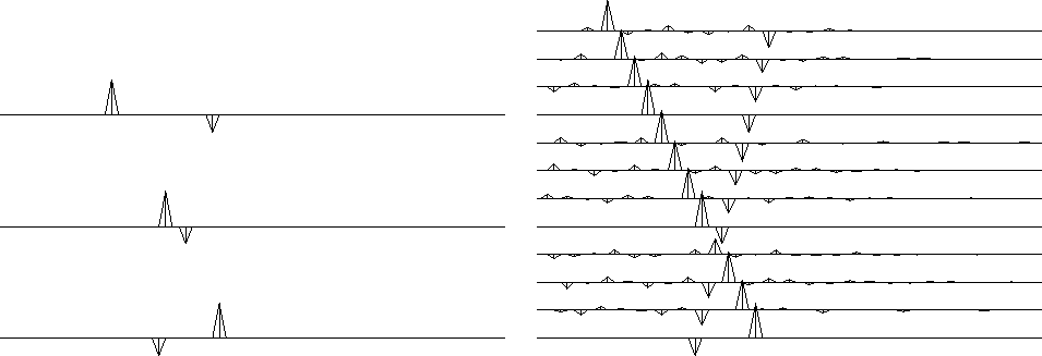
Let us now examine a case with minimal complexity. Figure 14 shows two plane waves recorded on three channels. That is the minimum number of channels required to distinguish two superposing plane waves. Notice on the interpolated data that the original traces are noise-free, but the new traces have acquired a low level of noise. This will be dealt with later.

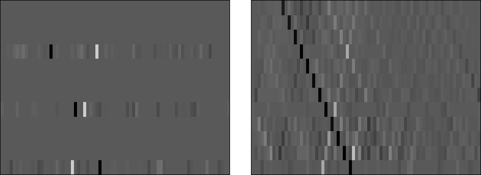
Figure 15 shows the same calculation in the presence of noise on the original data. We see that the noisy data is interpolatable just as was the noise-free data, but now we can notice the organization of the noise. It has the same slopes as the plane waves. This was also true on the earlier figures (Figure 13 and 14), as is more apparent if you look at the page from various grazing angles. To display the slopes more clearly, Figure 15 is redisplayed in a raster mode in Figure 16.

 

lacenoise
Figure 15 Interpolating noisy plane waves.

 

laceras
Figure 16 Interpolating noisy plane waves.