Lateral interpolation and extrapolation of a CMP gather

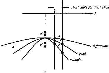
Practical problems dealing with common-midpoint gathers arise because of an insufficient number of traces. Truncation problems are those that arise because the geophone cable has a fixed length that is not as long as the distance over which seismic energy propagates. Figure 5 shows why cable truncations are a problem for conventional, ray-trace, stacking methods as well as for wave-equation methods.

 

nmotrunc
Figure 5 Normal moveout at the earth velocity brings the cable truncations on good events to a good place, causing no problems. The cable truncations of diffractions and multiples, however, move to a' and c', where they could be objectionable. Such corruption could make folly of sophisticated time-series analysis of the waveform found on a CDP stack.

Aliasing problems are those that arise because shots and geophones are not close enough together. Spatial aliasing of data on the offset axis seems to be a more serious problem for wave-equation methods than it is for ray-trace methods. The reason is that normal-moveout correction reduces the spatial frequencies. Gaps in the data, resulting from practical problems with the geophones, cable, and access to the terrain, are also frequently a snag.

Here these problems will all be attacked together with a systematic approach to estimating missing traces. The technique to be described is the simplest member of a more general family of missing data estimation procedures currently being developed at the Stanford Exploration Project.

First do normal-moveout correction, that is, stretch the time axis to flatten hyperbolas. The initial question is what velocity to use for the normal-moveout correction. For trace interpolation the appropriate moveout velocity turns out to be that of the dominating energy on the gather. On a given dataset this velocity could be primary velocity at some times and multiple velocity at other times. The reason for such a nonphysical velocity is this: the strong events must be handled well, in order to save the weak ones. Truncations of weak events can be ignored as a ``second-order'' problem. The practical problem is usually to suppress strong water-velocity events in the presence of weak sedimentary reflections, particularly at high frequencies. In principle, we might be seeking weak P-SV waves in the presence of strong P-P waves.

After NMO, the residual energy should have little dip, except of course where missing data, now replaced by zeroes, forces the existing data to be broad-banded in spatial frequency. In order to improve our view of this badly behaved energy, we pass the data through a ``badpass'' filter, such as the high-pass recursive dip filter.  

$${{k^2 \over -\,i \omega } \over \alpha \ \ +\ \ {k^2 \over -\,i \omega } }$$ (6)

Notice that this filter greatly weakens the energy with small k, that is, the energy that was properly moveout corrected. On the other hand, near the missing traces, notice that the spectrum should be broad-band with k and that such energy passes through the filter with almost unit gain.

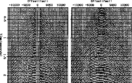
The output from the ``badpass'' filter is now ready to be subtracted from the data. The subtraction is done selectively. Where recorded data exists, nothing is subtracted. This completes the first iteration. Next the steps are repeated, and iterated. Convergence is finally achieved when nothing comes out of the badpass filter at the locations where data was not recorded. An example of this process can be found in Figure 6.

 

missfil
Figure 6 Field profile from Alaska with missing channels on the left (Western Geophysical), restored by iterative spatial filtering on the right. (Harlan)

The above procedure has ignored the possibility of dip in the midpoint direction.

This procedure is also limited because it ignores the possibility that several velocities may be simultaneously present on a dataset. To really do a good job of extending such a dataset may require a parsimonious model and a velocity spectral concept such as the ones developed later.