SAMPLED DATA AND Z TRANSFORMS

 

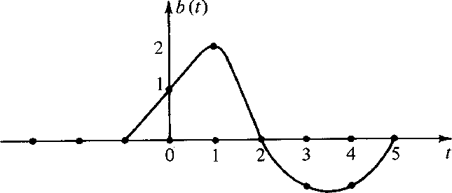1-1 Figure 1 A continuous time function sampled at uniform time intervals.

Consider the time function in Figure 1. To analyze such an observed time function in a computer it is necessary to approximate it in some way by a list of numbers. The usual way to do this is to evaluate or observe b(t) at a uniform spacing of points in time. For this example, such a digital approximation to the continuous function could be denoted by the vector

$$b_t \eq (\ldots\ 0,\, 0,\, 1,\, 2,\, 0,\, -1,\, -1,\, 0,\, 0,\, \ldots)$$ (1)

Of course if time points were taken more closely together we would have a more accurate approximation. Besides a vector, a function can be represented as a polynomial where the coefficients of the polynomial represent the values of b(t) at successive time points. In this example, we have  

$$B(Z) \eq 1 + 2Z + 0Z^2 - Z^3 - Z^4$$ (2)

This polynomial is called a Z transform. What is the meaning of Z in this polynomial? The meaning is not that Z should take on some numerical value; the meaning of Z is that it is the unit delay operator. For example the coefficients of ZB(Z) = Z + 2Z² - Z⁴ -Z⁵ are plotted in Figure 2. It is the same waveform as in Figure 1, but it has been delayed.

 

1-2 Figure 2 Coefficients of ZB(Z) are shifted version of the coefficients of B(Z)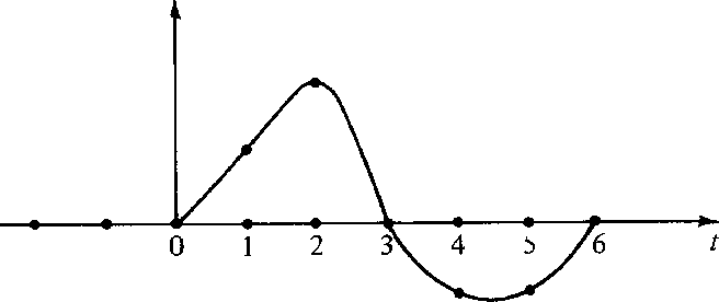

We see that the time function b_t is delayed n time units when B(Z) is multiplied by Zⁿ. The delay operator Z is very important in analyzing waves simply because waves take a certain amount of time to get from place to place.

Another value of the delay operator is that it may be used to build up more complicated time functions from simpler ones. Suppose b(t) represents the acoustic pressure function or the seismogram observed after a distant explosion. Then b(t) is called the impulse response. If another explosion occurs at t = 10 time units after the first, we expect the pressure function y(t) depicted in Figure 3.

 

1-3 Figure 3 Response to two explosions.

In terms of Z transforms this would be expressed as Y(Z) = B(Z) + Z¹⁰ B(Z). If the first explosion were followed by an implosion of half strength, we would have $B(Z) - {1\over 2}Z^{10}B(Z)$.If pulses overlap one another in time [as would be the case if B(Z) was of degree greater than 10], the waveforms would just add together in the region of overlap. The supposition that they just add together without any interaction is called the linearity assumption. This linearity assumption is very often true in practical cases. In seismology we find that--although the earth is a very heterogeneous conglomerations of rocks of different shapes and types--when seismic waves (of usual amplitude) travel through the earth, they do not interfere with one another. They satisfy linear superposition. The plague of nonlinearity arises from large amplitude disturbances. Nonlinearity does not arise from geometrical complications.

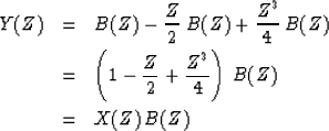
Now suppose there was an explosion at t = 0, a half-strength implosion at t = 1, and another, quarter-strength explosion at t = 3. This sequence of events determines a ``source'' time series, $x_t = (1, -{1 \over 2}, 0, {1 \over 4})$.The Z transform of the source is $X(Z) = 1 - {1 \over 2}Z + {1 \over 4}Z^3$.The observed y_t for this sequence of explosions and implosions through the seismometer has a Z transform Y(Z) given by

$$\begin{eqnarray} Y(Z) &= & B(Z) - {Z \over 2}\, B(Z) + {Z^3 \over 4}\, B(Z) \non... ...r 2} + {Z^3 \over 4} \right)\, B(Z) \nonumber \\ &= & X(Z)\, B(Z)\end{eqnarray}$$ (3)

The last equation illustrates the underlying basis of linear-system theory that the output Y(Z) can be expressed as the input X(Z) times the impulse response B(Z).

There are many examples of linear systems. A wide class of electronic circuits is comprised of linear systems. Complicated linear systems are formed by taking the output of one system and plugging it into the input of another. Suppose we have two linear systems characterized by B(Z) and C(Z), respectively. Then the question arises whether the two combined systems of Figure 4 are equivalent. The use of Z transforms makes it obvious that these two systems are equivalent since products of polynomials commute, i.e.,

$$\begin{eqnarray} Y_1(Z) &= & [X(Z) B(Z)]\, C(Z) = XBC \nonumber \\ Y_2(Z) &= & [X(Z) C(Z)]\, B(Z) = XCB = XBC\end{eqnarray}$$ (4)

 

1-4
Figure 4 Two equivalent filtering systems.

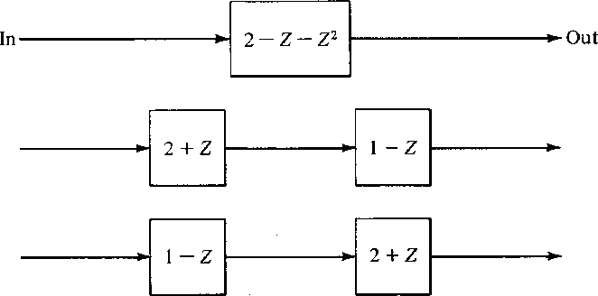
Consider a system with an impulse response B(Z) = 2 - Z - Z². This polynomial can be factored into $2 - Z - Z^2 = (2 + Z)\, (1 - Z)$,and so we have the three equivalent systems in Figure 5. Since any polynomial can be factored, any impulse response can be simulated by a cascade of two-term filters (impulse responses whose Z transforms are linear in Z).

 

1-5
Figure 5 Three equivalent filtering systems.

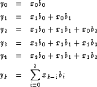
What do we actually do in a computer when we multiply two Z transforms together? The filter 2 + Z would be represented in a computer by the storage in memory of the coefficients (2, 1). Likewise, for 1 - Z the numbers (1, -1) are stored. The polynomial multiplication program should take these inputs and produce the sequence (2, -1, -1). Let us see how the computation proceeds in a general case, say

$$\begin{eqnarray} X(Z)\, B(Z) &= & Y(Z) \\ (x_0 + x_1 Z + x_2 Z + \cdots )\, (b_0 + b_1 Z + b_2 Z) &= & (y_0 + y_1 Z + y_2 Z^2 + \cdots )\end{eqnarray}$$ (5) (6)

Identifying coefficients of successive powers of Z, we get

$$\begin{eqnarray} y_0 &= & x_0 b_0 \nonumber \\ y_1 &= & x_1 b_0 + x_0 b_1 \nonum... ...3 b_1 + x_2 b_2 \nonumber \\ y_k &= & \sum^2_{i = 0} x_{k - i} b_i\end{eqnarray}$$ (7) (8)

Equation (8) is called a convolution equation. Thus, we may say that the product of two polynomials is another polynomial whose coefficients are found by convolution. A simple Fortran computer program which does convolution, including end effects on both ends, is this:

          DIMENSION X(LX), B(LB), Y(LY)
                  DO 10 IY=1,LY
          10      Y(IY) = 0.
                  DO 20 IX=1,NX
                  DO 20 IB=1,NB
                  IY = IX+IB-1
          20      Y(IY) = Y(IY) + X(IX)*B(IB)

The reader should notice that X(Z) and Y(Z) need not strictly be polynomials; they may contain both positive and negative powers of Z; that is

$$\begin{eqnarray} X(Z) &= & \cdots {x_{-2} \over Z^2} + {x_{-1} \over Z} + x_0 + ... ...\cdots {y_{-2} \over Z^2} + {y_{-1} \over Z} + y_0 + y_1 Z +\cdots\end{eqnarray}$$ (9) (10)

The effect of using negative powers of Z in X(Z) and Y(Z) is merely to indicate that data are defined before t = 0. The effect of using negative powers of Z in the filter is quite different. Inspection of (8) shows that the output y_k which occurs at time k is a linear combination of current and previous inputs; that is, $(x_i,\, i \leq k)$.If the filter B(Z) had included a term like b_-1/Z, then the output y_k at time k would be a linear combination of current and previous inputs and x_k+1, an input which really has not arrived at time k. Such a filter is called a nonrealizable filter because it could not operate in the real world where nothing can respond now to an excitation which has not yet occurred. However, nonrealizable filters are occasionally useful in computer simulations where all of the data are prerecorded.

EXERCISES:

1. Let B(Z) = 1 + Z + Z² + Z³ + Z⁴. Graph the coefficients of B(Z) as a function of the powers of Z. Graph the coefficients of $\left[ B(Z) \right]^2$.
2. If $x_t = \cos \omega_0 t$,where t takes on integral values, b_t = (b₀,b₁), and Y(Z) = X(Z)B(Z), what are A and B in $y_t = A \cos \omega_0 t + B \sin \omega_0 t$ ?
3. Deduce that, if $x_t = \cos \omega_0 t$ and $b_t = (b_0,\, b_1,\, \ldots,\, b_n)$, then y_t always takes the form $A \cos \omega_0 t + B \sin \omega_0 t$.