|
patchwt
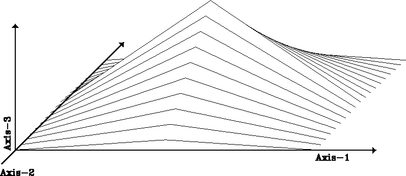
Figure 4 Patch weight. The weight function is applied to individual patches to prepare the patch for the linear interpolation of neighboring, overlapping patches. |  |
If done carelessly, the merging of individually processed patches in equation (2) can cause visible patch boundaries in the final image. I implemented Claerbout's1994 interpolation scheme, which linearly interpolates overlapping patches.
|
patchwt
Figure 4 Patch weight. The weight function is applied to individual patches to prepare the patch for the linear interpolation of neighboring, overlapping patches. |  |
Interpolation requires the application of weights to each data element. The weighting is easily implemented as the element-wise scaling of two vectors: one contains the data that is to be interpolated, the other one each element's corresponding weight. Algebraically, weighting of a vector amounts to a matrix multiplication by a diagonal matrix . The diagonal elements are the elements of the weight vector.
To interpolate the area of overlap linearly,
each patch ![]() is weighted
by a patch
is weighted
by a patch ![]() of identical size
but tent-like amplitudes (Figure 4).
Equation (3) expresses the weighting
as the multiplications of the diagonal matrices
of identical size
but tent-like amplitudes (Figure 4).
Equation (3) expresses the weighting
as the multiplications of the diagonal matrices ![]() .After zero padding and stacking the weighted patches by the row of
.After zero padding and stacking the weighted patches by the row of
![]() operators, the operator
operators, the operator ![]() is another weighting
operator that compensates for the variable amount of contributions every
output element received:
is another weighting
operator that compensates for the variable amount of contributions every
output element received:
![\begin{displaymath}
{\bf m}
=
{\bf W}_m
\left[
\begin{array}
{ccc}
{\bf Q}_1 ...
...}
{c}
{\bf m}_1 \\ {\bf m}_2 \\ {\bf m}_3 \\ \end{array}\right]\end{displaymath}](img24.gif) |
(3) |
How do we compute the operator ![]() ?
The same row of zero-padding operators
?
The same row of zero-padding operators ![]() that add the weighted patches
that add the weighted patches ![]() in equation (3)
adds the patch weights into a data quilt
in equation (3)
adds the patch weights into a data quilt ![]() .
.
![\begin{displaymath}
\hat{\bf w}_m
=
\left[
\begin{array}
{ccc}
{\bf Q}_1 & {\b...
...{array}
{c}
{\bf 1} \\ {\bf 1} \\ {\bf 1} \\ \end{array}\right]\end{displaymath}](img26.gif) |
(4) |
A user can modify the interpolation by supplying
any alternative weight function ![]() for the individual patches.
The algorithm will apply
the correct corresponding weight operator
for the individual patches.
The algorithm will apply
the correct corresponding weight operator ![]() .
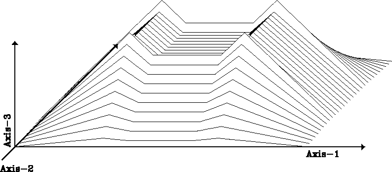
Figure 5 shows the weight vector
.
Figure 5 shows the weight vector ![]() that corresponds to four slightly separated tent weights
that corresponds to four slightly separated tent weights ![]() as shown in Figure 4.
as shown in Figure 4.
|
quiltwt
Figure 5 Superposition of overlapping patch weights. The shown quilt vector is used to balance the weighted patch contributions of the linear interpolation of neighboring, overlapping patches. The shown quilt vector is the result of zero padding and stacking of four slightly separated patch weights. The amplitudes indicate the number of weighted contributions each image quilt element received. The weighting operator |  |
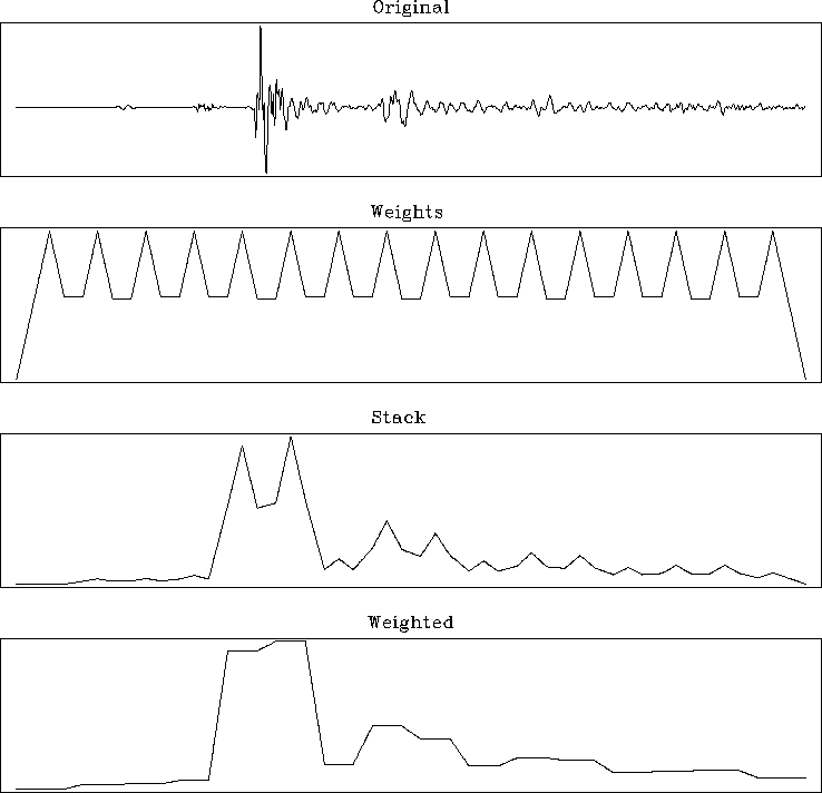
Figure 6 demonstrates the effect
of the weighted interpolation on the example in Figure 1.
The top panel shows the input trace. The bottom panel shows an estimate
of the signal's time variable variance.
The weight ![]() , shown in the second panel, correct the brute stack,
shown in the third panel, to the final result in the bottom panel.
, shown in the second panel, correct the brute stack,
shown in the third panel, to the final result in the bottom panel.
 |