

Next: 2-D TIME EXTRAPOLATION AND
Up: 1-D TIME EXTRAPOLATION AND
Previous: 1-D TIME EXTRAPOLATION AND
In this example the conjugate algorithm is tested
for a simple layered model.
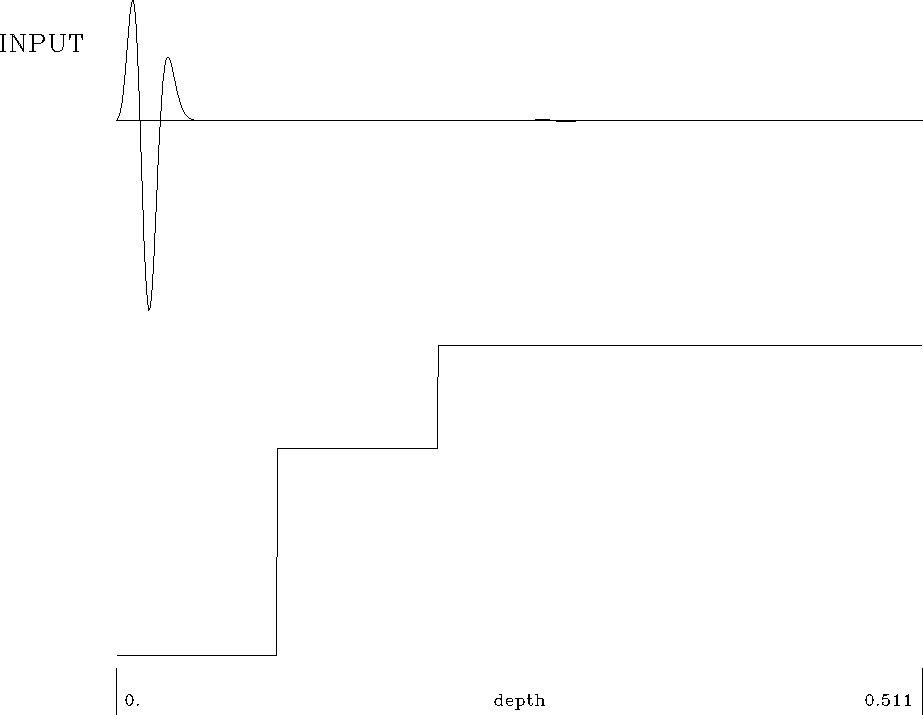
Figure ![[*]](http://sepwww.stanford.edu/latex2html/cross_ref_motif.gif) shows the velocity model and
the source function at time equals zero.
shows the velocity model and
the source function at time equals zero.
model
Figure 2 Input source wave field at time equals zero and
velocity function used for the model.
|
|  |

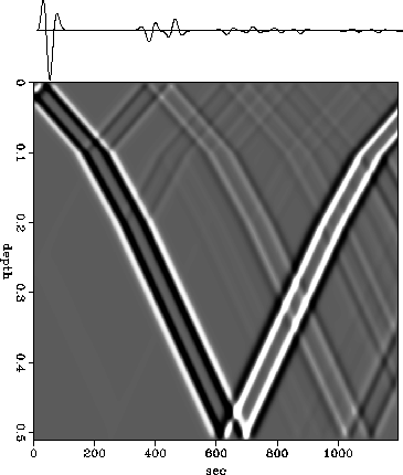
The result of the forward time-extrapolation
is shown in Figure ![[*]](http://sepwww.stanford.edu/latex2html/cross_ref_motif.gif) , on the top of the snap shots.
It contains the direct arrival,
primary reflection, ghost and multiple reflection events.
In order to avoid the inclusion of the boundary reflections,
time extrapolation was performed before the arrival time of the
boundary reflections (see the snap shots in Figure
, on the top of the snap shots.
It contains the direct arrival,
primary reflection, ghost and multiple reflection events.
In order to avoid the inclusion of the boundary reflections,
time extrapolation was performed before the arrival time of the
boundary reflections (see the snap shots in Figure ![[*]](http://sepwww.stanford.edu/latex2html/cross_ref_motif.gif) ).
Figure
).
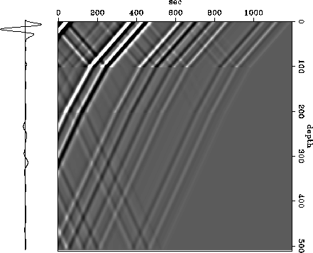
Figure ![[*]](http://sepwww.stanford.edu/latex2html/cross_ref_motif.gif) shows the result of the reverse-time
migration using the algorithm presented in this paper.
It can be seen that the conjugate operator does a good job.
The backprojected source wave field recovered closely matching the original
source function except for some artifacts.
These artifacts are mainly caused by the wave fields propagated downward,
and can be suppressed using a least-squares
optimization technique (Ji, 1992) by
solving an objective function as follows:
shows the result of the reverse-time
migration using the algorithm presented in this paper.
It can be seen that the conjugate operator does a good job.
The backprojected source wave field recovered closely matching the original
source function except for some artifacts.
These artifacts are mainly caused by the wave fields propagated downward,
and can be suppressed using a least-squares
optimization technique (Ji, 1992) by
solving an objective function as follows:
|  |
(8) |
where  represents the forward time-extrapolation operator in
equation (4), and
  and
and  are
the wave fields at depth equals zero and
at time equals zero, respectively.
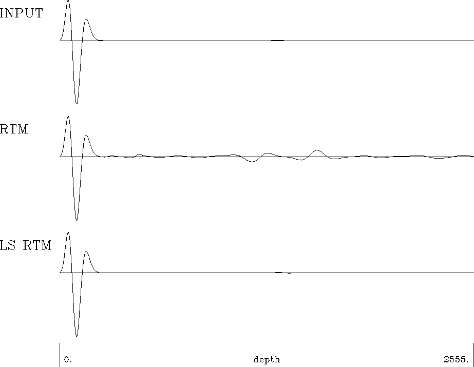
The result of the least-squares inversion is obtained
after 10 iterations using the conjugate gradient algorithm
and is shown in Figure
 ![[*]](http://sepwww.stanford.edu/latex2html/cross_ref_motif.gif) along with the original wave field
and the wave field obtained by the conjugate operator.
All the artifacts are well reduced in the least-squares inversion result.
frd
along with the original wave field
and the wave field obtained by the conjugate operator.
All the artifacts are well reduced in the least-squares inversion result.
frd
Figure 3 Forward time extrapolation experiment:
The time trace along with snap shots.
 rt
rt
Figure 4 Reverse time migration using the algorithm shown in
equation (2):
The depth section along with snap shots.

rtinv
Figure 5 Comparison of wave fields:
Top is the original wave field.
Middle is the result of conjugate operator.
Bottom is the result of the least-squares inversion
(after 10 iteration).
|
|  |


Next: 2-D TIME EXTRAPOLATION AND
Up: 1-D TIME EXTRAPOLATION AND
Previous: 1-D TIME EXTRAPOLATION AND
Stanford Exploration Project
11/17/1997

![[*]](http://sepwww.stanford.edu/latex2html/cross_ref_motif.gif) shows the velocity model and
the source function at time equals zero.
shows the velocity model and
the source function at time equals zero.

![[*]](http://sepwww.stanford.edu/latex2html/cross_ref_motif.gif) , on the top of the snap shots.
It contains the direct arrival,
primary reflection, ghost and multiple reflection events.
In order to avoid the inclusion of the boundary reflections,
time extrapolation was performed before the arrival time of the
boundary reflections (see the snap shots in Figure
, on the top of the snap shots.
It contains the direct arrival,
primary reflection, ghost and multiple reflection events.
In order to avoid the inclusion of the boundary reflections,
time extrapolation was performed before the arrival time of the
boundary reflections (see the snap shots in Figure ![[*]](http://sepwww.stanford.edu/latex2html/cross_ref_motif.gif) ).
Figure
).
Figure ![[*]](http://sepwww.stanford.edu/latex2html/cross_ref_motif.gif) shows the result of the reverse-time
migration using the algorithm presented in this paper.
It can be seen that the conjugate operator does a good job.
The backprojected source wave field recovered closely matching the original
source function except for some artifacts.
These artifacts are mainly caused by the wave fields propagated downward,
and can be suppressed using a least-squares
optimization technique (Ji, 1992) by
solving an objective function as follows:
shows the result of the reverse-time
migration using the algorithm presented in this paper.
It can be seen that the conjugate operator does a good job.
The backprojected source wave field recovered closely matching the original
source function except for some artifacts.
These artifacts are mainly caused by the wave fields propagated downward,
and can be suppressed using a least-squares
optimization technique (Ji, 1992) by
solving an objective function as follows:
![[*]](http://sepwww.stanford.edu/latex2html/cross_ref_motif.gif) along with the original wave field
and the wave field obtained by the conjugate operator.
All the artifacts are well reduced in the least-squares inversion result.
along with the original wave field
and the wave field obtained by the conjugate operator.
All the artifacts are well reduced in the least-squares inversion result.
