1-D TIME EXTRAPOLATION AND ITS CONJUGATE

In order to find a conjugate operator, the forward modeling operator must be formulated explicitly. The acoustic wave equation in the one dimensional space is

$${\partial^2 P \over {\partial t^2}} = v^2 {\partial^2 P \over {\partial z^2}},$$ (1)

where P is pressure field, v is the velocity, t and z are time and depth axis, respectively.

Approximating the derivatives by finite differences, equation (1) becomes

$${1 \over {\Delta t^2}}( P_{i-1,j} - 2 P_{i,j} + P_{i+1,j}) = {v_j^2 \over {\Delta z^2}}( P_{i,j-1} - 2 P_{i,j} + P_{i,j+1}),$$ (2)

where i and j represent time and depth indices, respectively. By rearranging equation (2) for time-extrapolation, we get the following equation:

$$P_{i+1,j} = 2(1-\alpha_j)P_{i,j} + \alpha_j(P_{i,j-1} + P_{i,j+1}) - P_{i-1,j}$$ (3)

$$\alpha_j = {v_j^2 \Delta t^2 \over {\Delta z^2}}$$

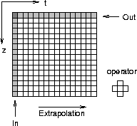
The differencing star in equation (3) covers the (t,z) space along the z-axis to extrapolate in time as shown schematically by Figure .

 

rt1dmdl Figure 1 Schematic for time extrapolation modeling for 1-D acoustic wave equation. The input is a source function at t=0 and the output is a trace at z=0.

To make the operator small enough to show on a page, I choose a small space like (t,z) = (4,5). The time extrapolation shown in equation (3) can be formulated algebraically as follows

$$\left[ \begin{array} {cccc} \bf S_1&\bf S_2&\bf S_3&\bf S_4\... ...y}\right] = \left[ \begin{array} {c} {\bf d}\end{array}\right],$$ (4)

where ${\bf m}$ is the model vector at t=1 with length 5, ${\bf d}$ is the data vector with length 4, and ${\bf I}$ and ${\bf 0}$ represent 5 by 5 identity and zero matrices. The matrix ${\bf T}$ in equation (4) represents tridiagonal matrix which looks like:

$$\left[ \begin{array} {ccccc} 2(1-\alpha_1)&\alpha_1&0&0&0\\ ... ...)&\alpha_4\\ 0&0&0&\alpha_5&2(1-\alpha_5)\\ \end{array}\right],$$ (5)

where $\alpha_j$ was shown in equation (3). The matrix ${\bf S}_i$ samples the wave field on the surface at i-th time and has the following form:

$${\bf S_1}= \left[ \begin{array} {ccccc} 1&0&0&0&0\\ 0&0&0&0&... ...1&0&0&0&0\\ 0&0&0&0&0\\ 0&0&0&0&0\\ \end{array}\right], \dots .$$ (6)

Now, reverse-time migration as the conjugate operator to the forward time-extrapolation becomes clear. It is obtained by transposing the operator in equation (4) and has the following form :

$$\left[ \begin{array} {cccc} \bf I&\bf 0&\bf 0&\bf 0\\ \end{a... ... = \left[ \begin{array} {c} {\bf \tilde m}\\ \end{array}\right]$$ (7)

where ${\bf T^*}$ and ${\bf S}_i^*$ are transpose matrices of ${\bf T}$ and ${\bf S}_i$.It is interesting that the conjugate algorithm follows the reverse-time extrapolation but with an operator which differs from the forward-time extrapolation. Instead of using wave fields from the two previous time steps together for an extrapolation, the conjugate operator uses the wave fields of the two previous time steps separately. The code for this algorithm, which has passed the dot-product test (Claerbout, 1992), is listed in the Appendix.