Observed Effect of Migration Velocity Changes

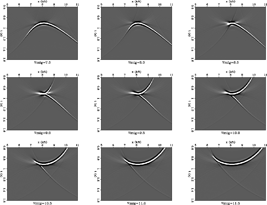
In practice, it is difficult to choose the correct velocity for migration. It is therefore instructive to see what effect the variation of migration velocity has in a v(x) medium. The synthetic data from Paper 1 are migrated with a Kirchhoff algorithm using various migration velocities and displayed in Figure 3. Each frame is migrated using a different constant velocity. The velocities used are 7.5 kft/s to 11.5 kft/s in increments of 0.5 kft/s. The image changes from undermigrated in the upper left corner to overmigrated in the lower right corner. The fourth frame (Vmig=9.0) is migrated with a velocity close to the RMS well velocity (8.84 kft/s) used in Figure 2.

As migration velocity is increased the image begins to develop an upper limb in the third frame (Vmig=8.5) of Figure 3. The plume is well formed in the fourth frame (Vmig=9.0) and then appears to rotate clockwise as migration velocity is increased. In the last frame the lower limb of the plume is very faint and the image looks overmigrated.

By scrutinizing the frames of the movie in Figure 3, we can see how the plume is formed. The left limb of the undermigrated image in frame 1 (Vmig=7.5) gets swept upward and becomes the upper limb of the plume in frame 4 (Vmig=9.0). Recall that the low velocity wedge (Figure 1) has the effect of making the left side of the true diffraction curve overmigrated and the right side undermigrated when the RMS well velocity is used. This overmigration sweeps the limb upwards. The right limb of the undermigrated image in frame 1 (Vmig=7.5) remains undermigrated as velocity increases until the last few frames where the typical overmigration ``smile'' begins to form.

 

movie
Figure 3 Kirchhoff migration with a range of velocities. The constant migration velocity ranges from 7.5 kft/s to 11.5 kft/s. The RMS well velocity at the diffractor position is 8.84 kft/s. If you have the electronic version of this report you can click on the button and see a movie of the image as a function of migration velocity. The movie begins with the true-diffraction curve as the first frame and then sweeps through the images for migration velocities ranging from 6.0 kft/s to 12.5 kft/s in steps of 0.5 kft/s.

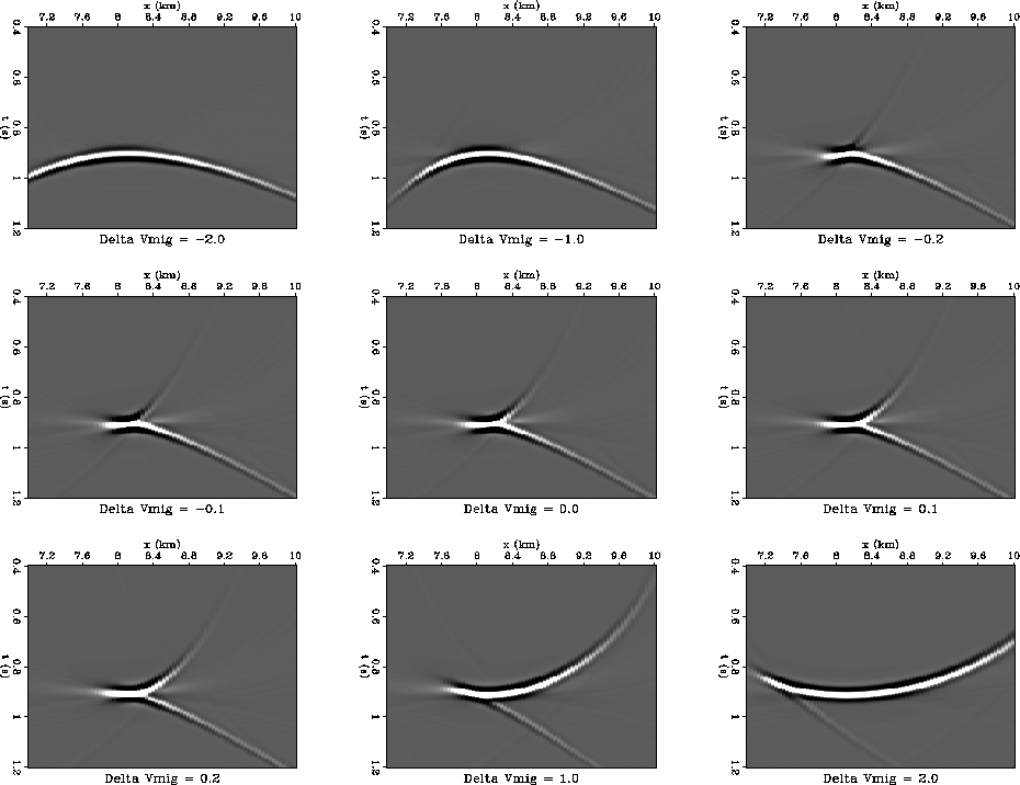
The nature of plume variation with migration velocity is examined for a different range of migration velocity with smaller increments of migration velocity variation around the RMS well velocity in Figure 4. The center frame ($\triangle V_{mig} =$0.0) is migrated with the RMS well velocity of 8.84 kft/s. The image in the first two frames is a characteristic undermigration ``frown'' and the image in the last frame is a characteristic overmigration ``smile''. As in Figure 3, we can see the left side of the diffraction curve being swept up to form the upper limb of the plume while the right side of the diffraction curve eventually forms the left side of the ``smile''. Migration velocities close to the RMS well velocity frames 3 ($\triangle V_{mig} =$-0.2) through 7 ($\triangle V_{mig} =$0.2) show the plume rotating slightly clockwise, although the overall rotation trend evident in frames 2 through 8 is somewhat counterclockwise.

 

kfrot
Figure 4 Kirchhoff migration with various migration velocities. The center frame is migrated with the RMS well velocity of 8.84 kft/s. The other frames are migrated with velocities of $V_{mig}=V_{rms well}+ \triangle V_{mig}$. The $\triangle V_{mig}$ values are given under the frame in units of kft/s.