


A good finite difference scheme should incorporate the relevant physical law into its representation. Extrapolating traveltimes is like propagating wavefronts; Huygens' principle and Fermat's principle should be respected. Extrapolating the gradients of traveltimes is like extending rays; Snell's law should be respected. Because these two extrapolations simulate the same physical phenomenon, the algorithm to do one can be translated and used to do the other. The algorithm described below does two extrapolations simultaneously.
|
vfdtime1
Figure 1 The grid and notations. | 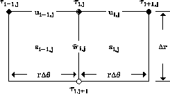 |


The eikonal equation in polar coordinates is as follows:
| |
(17) |
![]()
![[*]](http://sepwww.stanford.edu/latex2html/cross_ref_motif.gif) , I use
, I use According to Snell's law, the tangential component of the traveltime gradient to a boundary is continuous across the boundary. I define ui,j to be the tangential component of the traveltime gradient to the constant radius boundary. If we approximate the wavefront within a cell with a local plane wave, then we have
| |
(18) |
| |
(19) |
| |
(20) |
![]()
![]()
![]()
![]()
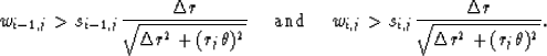 |
(21) |
![\begin{displaymath}
\Delta r = \min_{\hbox{all}\ i}[
r_j\Delta \theta \left\vert{w_{i,j} \over u_{i,j}}\right\vert],\end{displaymath}](img49.gif) |
(22) |
| (23) |
The implementation of this algorithm is quite simple and the program is fully
vectorizable. For example, the computation of ![]() for all i
can be coded as follows:
for all i
can be coded as follows:
        do i = 1,n
           sign1 = 0.5*(1.+sign(1.,u(i-1)))
           sign2 = 0.5*(1.+sign(1.,-u(i)))
           hatw1 = sign1*min(w(i-1),s(i))+(1.-sign1)*s(i-1)
           hatw2 = sign2*min(w(i),s(i-1))+(1.-sign2)*s(i)
           hatw(i) = min(hatw1,hatw2)
        enddo
One problem that has not been addressed yet is the possibility of refractions along the constant radius boundaries, which may initiate wave propagations toward the source. In practice, such situation seldom happen. To make the algorithm more complete, I handle such situation by adopting Podvin and Lecomte's method in polar coordinates and performing backward extrapolation as necessary. After obtaining the traveltimes in polar coordinates, I map them to Cartesian coordinates through interpolation.