Objective function

Suppose u₁(t) and u₂(t) are two traces of seismic data u(t,x):

$$u_1(t)=u(t,x_1),\ \ \ \ \ \ u_2(t)=u(t,x_2)$$

with $\Delta x = x_2-x_1$ being the distance between the two traces. We want to construct an objective function that measures the misfitting of two traces when they are shifted relative to one another. The standard least squares method suggests the following two expressions  

$$[u_1(t)-u_2(t+\tau)] ^2 \ \ \ \ \hbox{or} \ \ \ \ [u_2(t)-u_1(t-\tau)]^2.$$ (2)

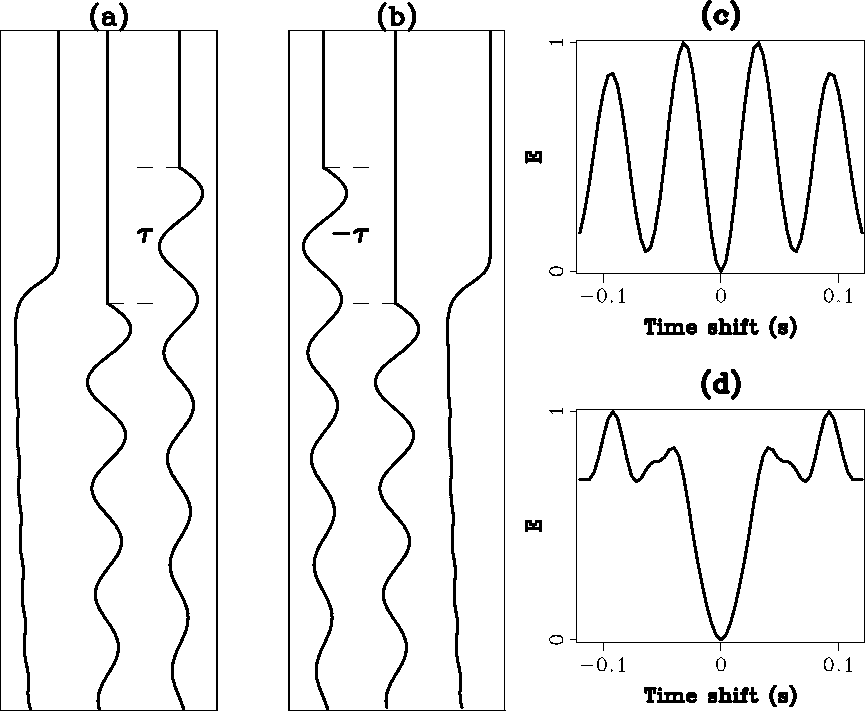
These two expressions are useful when seismic data is adequately sampled along the spatial axis. However, when data is aliased, these expressions as the functions of $\tau$, have many local minima, as shown in Figure 1c. This may lead to a totally wrong estimate of the time-shift $\tau$. The solution to this problem is to use some special information of data as constraints to reduce, or even to remove, the ambiguities.

There are many ways to constrain the solutions. The two commonly used methods are: adding extra terms to the objective function and multiplying weighting functions to the objective function. The method of adding extra terms can possibly preserve some of the important properties of the objective function, such as quadratic forms. But the relative weights between the two terms of the objective function are not easy to determine. The weighting method does not have this problem. But it will make the objective function non-quadratic when the weighting function are data-dependent. Since the expressions in equation (2) are not quadratic functions of time-shift $\tau$ anyway (thought they are quadratic functions of data), the weighting function method is apparently easy to apply.

Human eyes can eliminate the aliasing effects on dip-picking by looking at the amplitude information of data, especially the breaks of first arrivals. This suggests using the following objective function:  

$$E(\tau)={1 \over N} \sum^N_t\left\{ {1 \over \Vert u^2_1(t)\... ...2 {1 \over \Vert u^2_2(t)\Vert }[u_2(t)-u_1(t-\tau)]^2\right\},$$ (3)

where $\Vert u \Vert$ represents the smoothed version of u, and the summation is undertaken in the neighborhood of point (t,x). The reason to choose this kind of weighting function is clearly shown in Figures 1a and 1b. The penality is extremely large when the first breaks of traces do not match with each other. Figures 1a and 1b also show why both expressions in equation (2) must be included in the objective function. Figures 1c and 1d show that after the weighting functions are applied, false local minima become less ambiguous.

 

objill
Figure 1 Illustrations of the objective function: (a) three traces are $\Vert u^2_1(t) \Vert^{-1}$, u₁(t) and $u_2(t+\tau)$ from left to right, the weighting function $\Vert u^2_1(t) \Vert^{-1}$ causes the penalty to be extremely high when $\tau$ is not zero; (b) similar to (a) where three traces are $u_1(t-\tau)$, u₂(t) and $\Vert u^2_2(t) \Vert^{-1}$; (c) the objective function computed from traces in (a) and (b) without the weighting functions, it has several suspicious minima; (d) the objective function with the weighting functions, suspicious minima are lifted up.

An alternative form of the objective function is  

$$Q(p)={1 \over N} \sum^N_t\left\{ {1 \over \sqrt{\Vert u^2_1(... ...ert }} [u_1(t-{\tau \over 2})-u_2(t+{\tau \over 2})]^2 \right\}$$ (4)

which has one term and displays better symmetry around time t. But the disadvantage of this form is that the weighting function is $\tau$-dependent.