Angle-domain illumination gathers by wave-equation-based methods

Dip-dependent scattering-angle-domain illumination

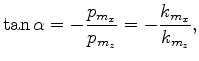
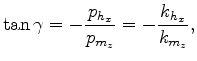
To overcome the limitation of the scattering-angle-domain illumination for planar reflectors discussed in the preceding section, we further decompose the illumination into dip-angle domain, resulting in dip-dependent scattering-angle-domain illumination. From equations 9 and 10, it is easy to obtain the tangent of the dip angle using either

$$\tan \alpha = - \frac{p_{m_x}}{p_{m_z}} = -\frac{k_{m_x}}{k_{m_z}},$$ (14)

or

$$\tan \alpha = \frac{p_{h_z}}{p_{h_x}} = \frac{k_{h_z}}{k_{h_x}},$$ (15)

where $k_{m_x}$ , $k_{m_z}$ and $k_{h_x}$ , $k_{h_z}$ are the horizontal and vertical components of the midpoint wavenumber vector and the subsurface-offset wavenumber vector, respectively.

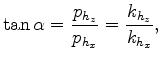Dip decomposition using either equation 14 or 15 has its own pros and cons. Equation 15 is suitable for computing dip-angle gathers for sparsely isolated image points, because it does not require any CMP information, i.e., $k_{mx}$ and $k_{mz}$ , and outputting gathers for sparsely isolated image points may mitigate the extra computer time and storage spent in computing both the horizontal and vertical subsurface offsets, $h_x$ and $h_z$ . On the other hand, equation 14 is computationally less demanding, because it does not require computing vertical subsurface offsets. However, it estimates dips using the CMP information, hence a block of densely sampled image points in the CMP domain should be output to avoid dip aliasing. In the following numerical examples, we use equation 14 for dip decomposition due to the fact that it is relatively inconvenient to output vertical subsurface offsets by using one-way wave-equation-based extrapolators.

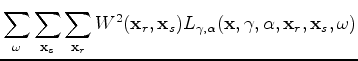
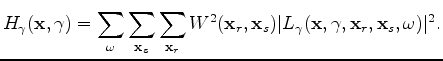
After transforming the subsurface-offset-domain sensitivity kernel into the dip-dependent scattering-angle domain, we can proceed to compute the corresponding Hessian using

$$H_{\gamma,\alpha}({\bf x},{\bf x}',\gamma,\gamma',\alpha,\alpha') = \sum_{\omega}\sum_{{\bf x}_s}\sum_{{\bf x}_r} W^2({\bf x}_r,{\bf x}_s) L_{\gamma,\alpha} ({\bf x},\gamma,\alpha,{\bf x}_r,{\bf x}_s,\omega)$$

$$\times L_{\gamma,\alpha}^{*}({\bf x}',\gamma',\alpha'{\bf x}_r,{\bf x}_s,\omega),$$ (16)

or the illumination using

$$H_{\gamma,\alpha}({\bf x},\gamma,\alpha) = \sum_{\omega}\sum_{{\b... ...ert L_{\gamma,\alpha}({\bf x},\gamma,\alpha,{\bf x}_r,{\bf x}_s,\omega)\vert^2,$$ (17)

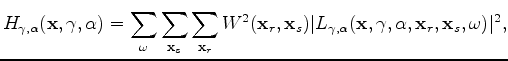where $L_{\gamma,\alpha}$ is the dip-dependent scattering-angle-domain sensitivity kernel. The complete procedure can be summarized as follows:

• for fixed ${\bf x}_s$ , ${\bf x}_r$ and $\omega$ , apply 3-D Fourier transform along axes $x$ , $z$ and $h_x$ (if only horizontal subsurface offsets are computed)
  

  $$L_{h}(x,z,h_x,{\bf x}_r,{\bf x}_s,\omega) \rightarrow L_{h}(k_x,k_z,k_{h_x},{\bf x}_r,{\bf x}_s,\omega),$$

  
  or along $z$ , $h_x$ and $h_z$ (if both horizontal and vertical subsurface offsets are computed)
  

  $$L_{h}(x,z,h_x,h_z,{\bf x}_r,{\bf x}_s,\omega) \rightarrow L_{h}(x,k_z,k_{h_x},k_{h_z},{\bf x}_r,{\bf x}_s,\omega);$$

  
  
• perform the mapping
  

  $$L_{h}(k_x,k_z,k_{h_x},{\bf x}_r,{\bf x}_s,\omega) \rightarrow L_{\gamma,\alpha}(k_x,k_z,\gamma,\alpha,{\bf x}_r,{\bf x}_s,\omega)$$

  
  according to relations 11 and 14, or
  

  $$L_{h}(x,k_z,k_{h_x},k_{h_z},{\bf x}_r,{\bf x}_s,\omega) \rightarrow L_{\gamma,\alpha}(x,k_z,\gamma,\alpha,{\bf x}_r,{\bf x}_s,\omega)$$

  
  according to relations 11 and 15;
• apply inverse 2-D Fourier transform along axes $k_x$ and $k_z$
  

  $$L_{\gamma,\alpha}(k_x,k_z,\gamma,\alpha,{\bf x}_r,{\bf x}_s,\omega) \rightarrow L_{\gamma,\alpha}(x,z,\gamma,\alpha,{\bf x}_r,{\bf x}_s,\omega),$$

  
  or inverse 1-D Fourier transform along axis $k_z$
  

  $$L_{\gamma,\alpha}(x,k_z,\gamma,\alpha,{\bf x}_r,{\bf x}_s,\omega) \rightarrow L_{\gamma,\alpha}(x,z,\gamma,\alpha,{\bf x}_r,{\bf x}_s,\omega)$$

  
  to obtain the dip-dependent scattering-angle-domain sensitivity kernel.
• compute either the dip-dependent scattering-angle-domain Hessian using equation 16 or the illumination using equation 17.

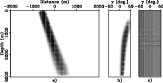
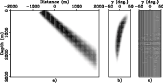
For the same constant velocity example, Figures 7 and 8 show the dip-dependent scattering-angle-domain illumination for $0^{\circ}$ and $-30^{\circ}$ dip angles, respectively. The acquisition geometry is the same as that in Figure 5, i.e., $1$ shot and $401$ receivers. The illumination gathers (Figures 7(b) and 8(b)) successfully predict the angle-dependent illumination for both the horizontal and dipping reflectors (Figure 7(c) and Figure 8(c)).

const-imag-hess-dip-adcig1
Figure 7. Dip-dependent scattering-angle-domain illumination. Panel (a) is the illumination for a constant dip angle $\alpha =0^{\circ }$ and a constant scattering angle $\gamma =18.75^{\circ }$ ; (b) is the illumination angle gather for a constant dip angle $\alpha =0^{\circ }$ and at spatial location $x=0$ m; (c) is the reflectivity angle gather for the horizontal reflector extracted a $x=0$ m, it is the same as Figure 6(a). [CR]

const-imag-hess-dip-adcig2
Figure 8. Dip-dependent scattering-angle-domain illumination. Panel (a) is the illumination for a constant dip angle $\alpha =-30^{\circ }$ and a constant scattering angle $\gamma =18.75^{\circ }$ ; (b) is the illumination angle gather for a constant dip angle $\alpha =-30^{\circ }$ and at spatial location $x=0$ m; (c) is the reflectivity angle gather for the dipping reflector extracted at $x=0$ m, it is the same as Figure 6(b). [CR]

Angle-domain illumination gathers by wave-equation-based methods