|
|
|
|
Mechanics of stratified anisotropic poroelastic media |
Now I assume throughout the rest of the paper that the porous layers are stacked vertically (![]() - or
- or ![]() -axis) and for this geometry
it is easy to see that the three horizontal strains
-axis) and for this geometry
it is easy to see that the three horizontal strains ![]() ,
, ![]() , and
, and ![]() must be continuous if the layers are in solid-welded contact. Furthermore, the vertical stress
must be continuous if the layers are in solid-welded contact. Furthermore, the vertical stress
![]() , and rotational stresses
involving the vertical direction
, and rotational stresses
involving the vertical direction
![]() and
and
![]() must also be continuous. These conditions are equivalent to
an assumption of welded contact between layers. If contact is not welded, then the system can have more complicated behaviors
than those being considering here.
must also be continuous. These conditions are equivalent to
an assumption of welded contact between layers. If contact is not welded, then the system can have more complicated behaviors
than those being considering here.
Appendix A summarizes the Backus (1962) and/or Schoenberg and Muir (1989) approach to elastic layer averaging. The method I present here provides a small generalization of this approach, taking the presence of the pore-fluid into account. For the drained situation, the influence of the fluid on the system mechanics is minimal (as will be shown). But I should nevertheless have this result available to compare it with the more interesting case of the undrained layers.
Although the shear moduli normally associated with the twisting shear components ![]() ,
, ![]() , and
, and ![]() usually do not
interact with the pore-fluid itself in systems as symmetric or more symmetric than orthotropic, I nevertheless need
to carry these terms along in the poroelastic formulation for layered systems because of possible boundary effects due to
welded contact at interfaces. To accomplish this goal, I will generalize the form of equation (42) from Appendix A.
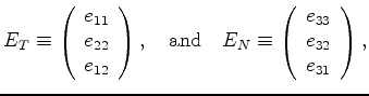
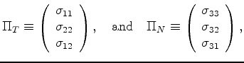
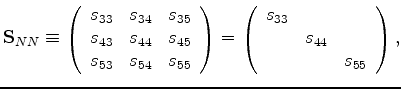
In compliance form, the equations will relate the strains
usually do not
interact with the pore-fluid itself in systems as symmetric or more symmetric than orthotropic, I nevertheless need
to carry these terms along in the poroelastic formulation for layered systems because of possible boundary effects due to
welded contact at interfaces. To accomplish this goal, I will generalize the form of equation (42) from Appendix A.
In compliance form, the equations will relate the strains
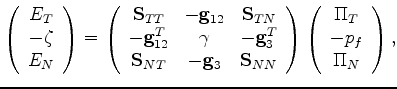
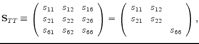
The required general relationship is:
 (the
(the
All the poroelastic contributions to (29) are determined by ![]() ,
,
![]() ,
and
,
and ![]() .
The scalar
.
The scalar ![]() within the
within the ![]() matrix in (29)
was defined earlier in (8), and is the only term in the
matrix in (29)
was defined earlier in (8), and is the only term in the ![]() matrix
that includes fluid effects directly through
matrix
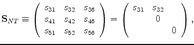
that includes fluid effects directly through ![]() . The remaining pair of vectors contained within the
. The remaining pair of vectors contained within the ![]() matrix
in (29) is defined by:
matrix
in (29) is defined by:
I now consider two examples of special uses of the general equation (29)
for different choices of boundary conditions. These two physical circumstances covered in the
cases considered are distinct end-members. For relatively high-frequency wave propagation, it is appropriate to consider that
the fluids do not have time to equilibrate, and therefore fluid pressures can be different in distinct layers,
while the fluid particles do not have time to move very far during wave passage time, so the fluid increment
![]() essentially everywhere. This situation is called the ``undrained'' condition. An alternative condition
is the fully drained condition, in which the fluid particles have as much time as they need to achieve
fluid-pressure equilibration, so that
essentially everywhere. This situation is called the ``undrained'' condition. An alternative condition
is the fully drained condition, in which the fluid particles have as much time as they need to achieve
fluid-pressure equilibration, so that ![]() constant. These two limiting situations are clearly connected
physically via Darcy's law, which provides the mechanism to move fluid particles, and ultimately to guarantee that the fluid
pressure reaches an equilibrium state. Bringing Darcy's law actively into oplay in the equations would
result in Biot-style equations which are beyond my current scope. So I consider only the end-member conditions
for the present contribution.
constant. These two limiting situations are clearly connected
physically via Darcy's law, which provides the mechanism to move fluid particles, and ultimately to guarantee that the fluid
pressure reaches an equilibrium state. Bringing Darcy's law actively into oplay in the equations would
result in Biot-style equations which are beyond my current scope. So I consider only the end-member conditions
for the present contribution.
|
|
|
|
Mechanics of stratified anisotropic poroelastic media |