Selecting the right hardware for Reverse Time Migration

Implementing RTM on FPGAs

The core computation of RTM is finite-difference-based 3D convolutions, which normally perform multiplications and additions on a number of adjacent points. While the points are neighbors to each other in a 3D geometric perspective, they are often stored relatively far apart in memory. For example, in the 7-point 2D convolution performed on a 2D array shown in Figure 7, data items $(0,3)$ and $(1,3)$ are neighbors in the $y$ direction. However, suppose the array uses a row-major storage and has a row size of 512, the storage locations of $(0,3)$ and $(1,3)$ will be 512 items (one line) away. For a 3D array of the size $512\times512\times512$, the neighbors in the $z$ direction will be $512\times 512$ items (one slice) away. In software implementations, this memory storage pattern can incur a lot of cache misses when the domain gets larger, and decreases the efficiency of the computation.

convolution-2D
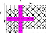
Figure 7. A streaming example of 2D convolution.[NR]

In an FPGA implementation, we use BRAMs to store a window of the input stream and enable the circuit to compute one result per cycle. Figure 7 demonstrates this concept. Suppose we are applying the stencil on the data item $(3,3)$, meaning the circuit requires 13 different values (shown in red). As the data items are streamed in one by one, in order to make the values from $(0,3)$ to $(6,3)$ available to the circuit, we use BRAMs to buffer the window of all the six lines of input values from $(0,3)$ to $(6,3)$ (shown in grey grid). In the next cycle, the first value $(0,3)$ pops out of the window, as $(0,3)$ is no longer needed for the following computation. Meanwhile, the next value $(6,4)$ is pushed into the window buffer, as $(6,4)$ is needed for the next stencil operation.

Considering the BRAMs as the `cache' of an FPGA design, the above window buffer mechanism provides a perfect `cache' behavior: firstly, the data item gets streamed into the window buffer at exactly the cycle that the data item is needed for the computation for the first time; secondly, the data item only resides in the window buffer for the period of time that the data item is needed for the computation. Current BRAMs can hold 6MB of data, or 1.5 million elements, when the data is stored as float. The window size that needs to be buffered is proportional to $n1*n2*no$, where $no$ is the spatial derivative approximation. For large data volumes and high order stencils, this exceeds current BRAM storage, requiring domain decomposition. The size of BRAM tends to follow Moore's Law, doubling every 18 months.

Selecting the right hardware for Reverse Time Migration