 |
 |
 |
 | 3D shot-profile migration in ellipsoidal coordinates |  |
![[pdf]](icons/pdf.png) |
Next: Impulse Response Tests
Up: 3D Implicit Finite-difference Propagation
Previous: 3D Implicit Finite-difference Propagation
Using the 4th-order approximation is equivalent to solving a cascade
of partial differential equations (, )
We solve these equations implicitly at each
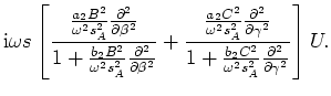 extrapolation step
by a finite-difference splitting method that alternately
advances the wavefield in the
extrapolation step
by a finite-difference splitting method that alternately
advances the wavefield in the  and
and  directions.
Splitting methods allow us to apply the
directions.
Splitting methods allow us to apply the  and
and  scaling factors
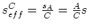
directly by introducing rescaled effective slowness models:
scaling factors
directly by introducing rescaled effective slowness models:
 and
and
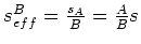 .
.
One drawback to splitting methods is that they generate numerical
anisotropy. To minimize these effects, we apply a Fourier-domain phase-correction
filter (, )
 |
(A-14) |
where
![$\displaystyle k_L = \sqrt{ 1-\frac{k_\beta^2}{(\omega s_B^r)^2} -\frac{k_\gamma...
...a}{\omega s_A^r})^2}{1-b_i ( \frac{k_\gamma}{\omega s_A^r})^2} \right) \right],$](img84.png) |
(A-15) |
and 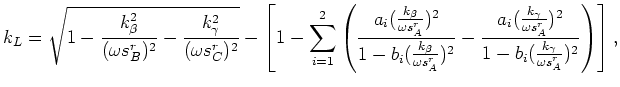 and
and  are reference slownesses chosen to be the
mean value of
are reference slownesses chosen to be the
mean value of  and
and  defined above.
|
|
|
|
| 3D shot-profile migration in ellipsoidal coordinates | |
|
Next: Impulse Response Tests
Up: 3D Implicit Finite-difference Propagation
Previous: 3D Implicit Finite-difference Propagation
2009-04-13

![$\displaystyle {\rm i} \omega s
\left[
\frac{ \frac{a_2 B^2}{\omega^2s_A^2} \fra...
...1+\frac{b_2C^2}{\omega^2s_A^2}\frac{\partial^2}{\partial \gamma^2} }
\right] U.$](img79.png)