3D shot-profile migration in ellipsoidal coordinates

3D Implicit Finite-difference Propagation

A general approach to 3D implicit finite-difference propagation is to approximate the square-root by a series of rational functions (, )

$$S_\alpha = \sqrt{1 - B^2 S_\beta^2 - C^2 S_\gamma^2} \approx \sum_{i=1}^{n} \frac{ a_i S_r^2}{1-b_i S_r^2},$$ (A-11)

where $S_i= \frac{k_i}{\omega s_A}$ for $i=\alpha,\beta,\gamma$, term $S_r^2=B^2S_\beta^2 + C^2 S_\gamma^2$, and $n$ is the order of the coefficient expansion. At this point, we do not address the anisotropy generated by the $B$ and $C$ coefficients, as they can be implemented through additional slowness model stretches.

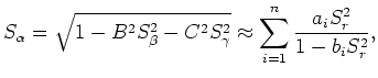
One procedure for finding an optimal set of coefficients is to solve the following optimization problem (, ),:

$${\rm min} \int_{0}^{{\rm sin} \phi} \left[ \sqrt{1-S_r^2} - \sum_{i=1}^{n} \frac{a_i S_r^2}{1 - b_i S_r^2} \right]^2 {\rm d}S_r,$$ (A-12)

where 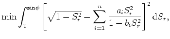$\phi$ is the maximum optimization angle. We generated the following results using a 4th-order approximation and coefficients found in Table 1 (Lee and Suh, 1985).

Table 1: Coefficients used in 3D implicit finite-difference wavefield extrapolation.

Coeff. order $i$	Coeff. $a_i$	Coeff. $b_i$
1	0.040315157	0.873981642
2	0.457289566	0.222691983

3D shot-profile migration in ellipsoidal coordinates