Angle-domain common-image gathers in generalized coordinates

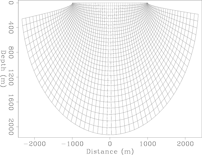
Elliptic Coordinates

The elliptic coordinate system (see figure 3) is defined by

$$\left[ \begin{array}{c} x_1\\ x_3 \end{array} \right] = \left[ \... ...os} \,\xi_1\\ a\, {\rm sinh}\, \xi_3 \, {\rm sin} \,\xi_1 \end{array} \right].$$ (20)

The transformation matrix is defined by

$$\left[ \begin{array}{cc} \frac{\partial x_1}{\partial \xi_1}& \fr... ...{\rm cos} \,\xi_1 & {\rm cosh} \,\xi_3 \, {\rm sin} \,\xi_1 \end{array}\right],$$ (21)

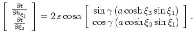
which leads to the following differential travel-time equations

$$\left[ \begin{array}{c} \frac{\partial t}{\partial h_{\xi_1}}\\ ... ...gamma \,( a \, {\rm cosh} \, \xi_3 \, {\rm sin} \, \xi_1 ) \end{array} \right].$$ (22)

The computation for the ADCIG in elliptic coordinates is given by

$${\rm tan}\,\gamma =- \frac{\partial \xi_3}{\partial h_{\xi_1}}.$$ (23)

Thus, ADCIGs calculated in elliptic coordinates directly yield the reflection opening angle without any additional filtering.

EC Figure 3. Example of an elliptic coordinate system. [NR]

Angle-domain common-image gathers in generalized coordinates