Angle-domain common-image gathers in generalized coordinates

Numerical Examples

This section presents a numerical test of the generalized theory by comparing ADCIGs from Cartesian and elliptic coordinate systems for the BP synthetic velocity model. () demonstrate that the elliptic coordinate system does not induce an anisotropic wavenumber stretch during wavefield extrapolation. I assert that equation 23 is a similar expression, and is a further argument that the Cartesian and elliptic coordinate ADCIGs should yield similar results. (The results are not necessarily equal due to the differing wavefield extrapolation accuracy.)

The numerical examples presented herein were generated using a shot-profile migration algorithm with extrapolation operators accurate to roughly 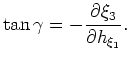$80^\circ$ (Lee and Suh, 1985). For each profile I did the following: i) computed 31 subsurface shifts at each extrapolation step; ii) calculated ADCIGs using the procedure described in Sava and Fomel (2003); and iii) interpolated the single-shot ADCIG output to the global image volume.

The top and bottom panels of figure 4 show the image volumes for the elliptic and Cartesian coordinate systems, respectively. I indicate a number of locations where the elliptic coordinate system produces superior images.

Images
Figure 4. Comparative BP velocity model images for the elliptic (top panel) and Cartesian (bottom panel) coordinate systems.[CR]

Figure 5 shows the ADCIGs corresponding to figure 4 for the elliptic (top panel) and Cartesian (bottom panel) coordinate systems. The ADCIGs are spaced out every 500 meters, and have an angular bandwidth of $[-60^\circ < \gamma < 60^\circ]$.

EllipticADCIG
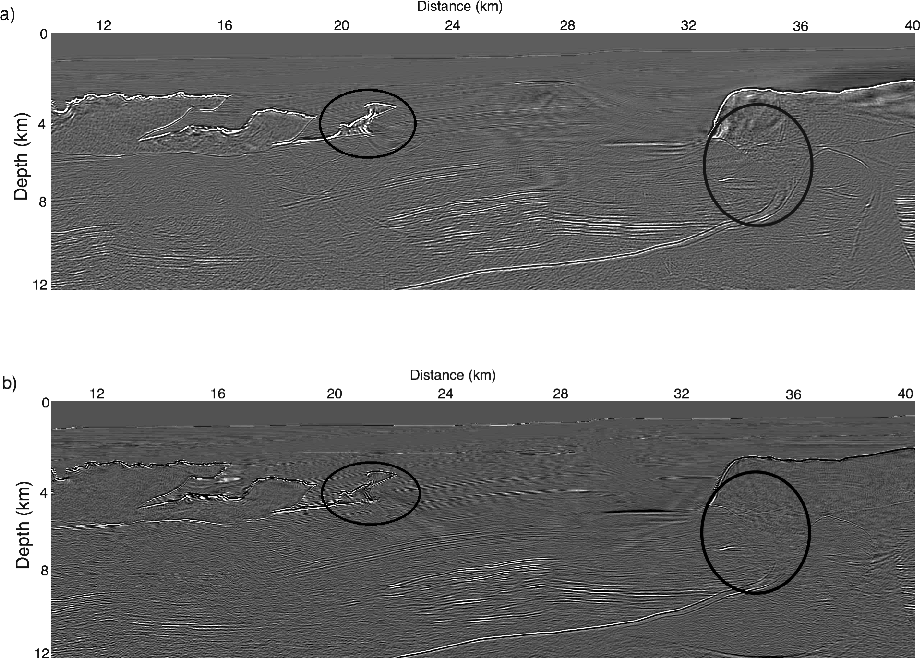
Figure 5. ADCIGs corresponding to the images in figure 4 calculated in the elliptic coordinates.[CR]

Note that the ADCIGs are flat, though with slightly different amplitudes caused by differing illumination. The similarity between these gathers indicates the validity of the general coordinate ADCIG theory.

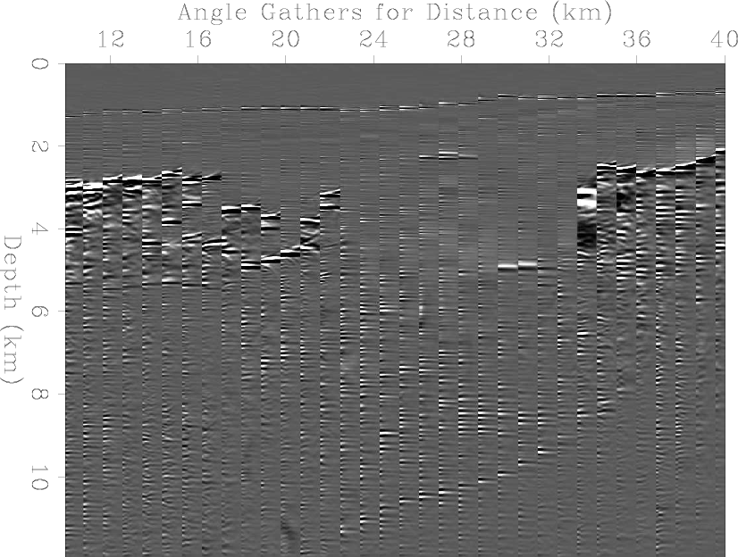
A second test that illustrates the validity of this approach is to examine how the ADCIGs change when the velocity profile is altered. For this test, we rescale the BP synthetic velocity profile by factors from 0.92x to 1.08x in increments of 0.02x and migrate a single shot-profile. Figure 6 presents the elliptic coordinate ADCIG results for an ADCIG and shot point coincidentally located at 12000 m.

Nice
Figure 6. Single shot-profile migration ADCIGs for a coincident ADCIG and source point at 12000 m. Note that the image is best focused when the correct velocity is used, and frowns and smiles are observed when migration velocity is used. [ER]

As we progress from the leftmost (too slow) to the rightmost (too fast) panels, we observe that the imaged reflections go from smiling to frowning. As expected, the ADCIG is most flat and well-focused where the true velocity model is used.

Angle-domain common-image gathers in generalized coordinates