|
|
|
|
Angle-domain common-image gathers in generalized coordinates |
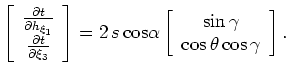
![$\displaystyle \left[ \begin{array}{c}
x_1\\
x_3
\end{array} \right] =
\left[ \...
...\end{array}\right]
\left[ \begin{array}{c}
\xi_1 \\
\xi_3
\end{array} \right],$](img44.png) |
(16) |
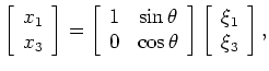 is the shearing angle. The transformation matrix is
| (17) |
![$\displaystyle \left[ \begin{array}{c}
\frac{\partial t}{\partial h_{\xi_1}}\\
...
...} \, \gamma \\
{\rm cos} \, \theta \, {\rm cos} \, \gamma
\end{array} \right].$](img47.png) |
(18) |
 in order to recover the true
reflection opening angle.
in order to recover the true
reflection opening angle.
|
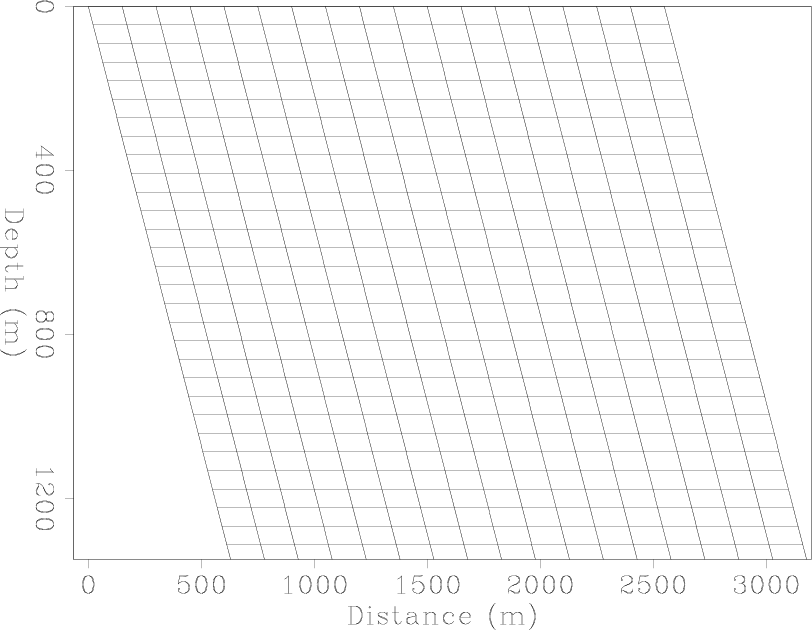
Sheared
Figure 2. Example of a sheared Cartesian coordinate system with a shear angle of 25 |
|
|---|---|
|
|
|
|
|
|
Angle-domain common-image gathers in generalized coordinates |