Angle-domain common-image gathers in generalized coordinates

Cartesian Coordinates

A Cartesian coordinate system $\boldsymbol{x}$ can be defined from a unit square $\boldsymbol{\xi}$ by

$$\left[ \begin{array}{c} x_1\\ x_3 \end{array} \right] = \left[ \... ...\end{array}\right] \left[ \begin{array}{c} \xi_1 \\ \xi_3 \end{array} \right].$$ (12)

The partial differential transformation matrix is

$$\left[ \begin{array}{cc} \frac{\partial x_1}{\partial \xi_1}& \fr... ...d{array} \right] = \left[ \begin{array}{cc} a & 0 \\ 0 & b \end{array}\right],$$ (13)

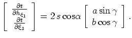
leading to the following differential travel-time equations

$$\left[ \begin{array}{c} \frac{\partial t}{\partial h_{\xi_1}}\\ ... ...}{c} a \, {\rm sin} \, \gamma \\ b \, {\rm cos} \, \gamma \end{array} \right].$$ (14)

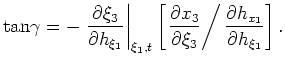
The Cartesian ADCIG computation is given by

$${\rm tan}\gamma = - \frac{b}{a} \frac{\partial \xi_3}{\partial h_{\xi_1}}.$$ (15)

Note that where the axes are equally sampled, one recovers the correct reflection opening angle; situations where the axes are not equally sampled require an additional scaling. This stretch is usually taken into account during the Fourier transformation implicit in equation 7.

Angle-domain common-image gathers in generalized coordinates