|
|
|
|
With ideal data, attenuating both specular and diffracted
multiples could, in principle, be accomplished simply by zeroing out
(with a suitable taper) all the ![]() -planes
except
-planes
except ![]() in the model cube
in the model cube
![]() and taking the inverse apex-shifted Radon transform.
In practice, however, the primaries may not be well-corrected
and primary energy may map to a other nearby
and taking the inverse apex-shifted Radon transform.
In practice, however, the primaries may not be well-corrected
and primary energy may map to a other nearby ![]() -planes. Energy from
the multiples may also map to those planes and so we have the usual
trade-off of primary preservation versus multiple attenuation. The
advantage of the apex-shift transform is that the diffracted multiples
are well focused to their corresponding
-planes. Energy from
the multiples may also map to those planes and so we have the usual
trade-off of primary preservation versus multiple attenuation. The
advantage of the apex-shift transform is that the diffracted multiples
are well focused to their corresponding  -planes instead of being
mapped as unfocused noise that interferes with the primaries.
-planes instead of being
mapped as unfocused noise that interferes with the primaries.
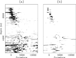
To illustrate the mapping of the primaries, the specular multiples
and the diffracted multiples, between the image space ![]() and the
apex-shifted Radon space
and the
apex-shifted Radon space ![]() , I chose the ADCIG in
Figure 15(a). Although this ADCIG
shows no discernible primaries below the salt, it nicely shows the apex-shifted
moveout of the diffracted multiples. This ADCIG was transformed to the Radon
domain with the apex-shifted transform described by equations 28
and 29. The kernel of the Radon transform is given by equation
27 and I applied the Cauchy regularization given in equation
31.
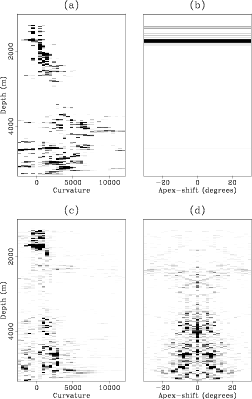
Figure 16 shows envelopes of the data in the Radon domain.
Panel (a) shows the
, I chose the ADCIG in
Figure 15(a). Although this ADCIG
shows no discernible primaries below the salt, it nicely shows the apex-shifted
moveout of the diffracted multiples. This ADCIG was transformed to the Radon
domain with the apex-shifted transform described by equations 28
and 29. The kernel of the Radon transform is given by equation
27 and I applied the Cauchy regularization given in equation
31.
Figure 16 shows envelopes of the data in the Radon domain.
Panel (a) shows the ![]() plane from the
plane from the ![]() volume.
This plane corresponds to zero apex-shift and therefore this is where the majority
of the specular multiples should map. Figure 16(b) shows the
zero-curvature
volume.
This plane corresponds to zero apex-shift and therefore this is where the majority
of the specular multiples should map. Figure 16(b) shows the
zero-curvature ![]() plane, that is, the plane where the primaries should map.
Notice that since the primaries are flat, they are independent of the apex-shift
and therefore map as flat lines on this plane. Notice also that there are no
significant primaries on the ADCIG below 2000 m. For comparison,
Figure 16(c) shows the
plane, that is, the plane where the primaries should map.
Notice that since the primaries are flat, they are independent of the apex-shift
and therefore map as flat lines on this plane. Notice also that there are no
significant primaries on the ADCIG below 2000 m. For comparison,
Figure 16(c) shows the ![]() deg plane. This corresponds to the
apex-shift of the most obvious diffracted multiple and we see its energy mapped
on this plane at about 4000 m. Finally, Figure 16(d) shows a
plane at a large curvature,
deg plane. This corresponds to the
apex-shift of the most obvious diffracted multiple and we see its energy mapped
on this plane at about 4000 m. Finally, Figure 16(d) shows a
plane at a large curvature, ![]() m/deg. Notice the energy from the diffracted
multiple at approximately
m/deg. Notice the energy from the diffracted
multiple at approximately ![]() deg.
deg.
|
|---|
|
envelopes
Figure 16. Different views from the cube of the apex-shifted transform for the ADCIG at 6744 m. (a): zero apex-shift plane. (b) zero curvature plane. (c): plane at apex shift |
|
|
It is important to emphasize the difference between the standard transform and
the apex-shifted transform. While the ![]() plane of the apex-shifted transform
is similar to the standard transform, they are not the same, as shown in
Figure 17. Both panels in this figure are plotted with the exact
same plotting parameters. Primaries are mapped near the
plane of the apex-shifted transform
is similar to the standard transform, they are not the same, as shown in
Figure 17. Both panels in this figure are plotted with the exact
same plotting parameters. Primaries are mapped near the ![]() line in both
planes while specular multiples are mapped to other
line in both
planes while specular multiples are mapped to other ![]() values.
Notice how in the standard transform Figure 17(a), the
diffracted-multiple energy is mapped as background noise,
especially at the largest positive and negative
values.
Notice how in the standard transform Figure 17(a), the
diffracted-multiple energy is mapped as background noise,
especially at the largest positive and negative ![]() values. In the
values. In the ![]() plane
of the apex-shifted transform (panel (b)), however, the diffracted multiples are
not present since their moveout apex is not zero. These multiples, therefore,
do not obscure the mapping of the specular multiples. Notice also
that the primary energy is much lower than in Figure 17(a) since
in the apex-shifted transform the primary energy is mapped not only to the
plane
of the apex-shifted transform (panel (b)), however, the diffracted multiples are
not present since their moveout apex is not zero. These multiples, therefore,
do not obscure the mapping of the specular multiples. Notice also
that the primary energy is much lower than in Figure 17(a) since
in the apex-shifted transform the primary energy is mapped not only to the
![]() plane but to other planes as well as illustrated previously in
Figure 16(b).
plane but to other planes as well as illustrated previously in
Figure 16(b).
|
|---|
|
radon-comp
Figure 17. Radon transforms of the ADCIG in Figure 15b. (a): standard 2D transform. (b): |
|
|
|
|
|
|