Projecting data samples along the path

After path $\vec{x}(t)$ is calculated from the sample points, proper data processing is still required to clearly display the path. The path has only has length but no volume, making it nearly invisible. Thus, the path must attain some volume. A straightforward approach is to define a spherical neighborhood around the path. For each point $\vec{x}(t)$, let the neighborhood be

$$\begin{eqnarray} N(x(t),R) = \{\vec{x}(\tau) : \vert\vert\vec{x}(t)-\vec{x}(\tau)\vert\vert \le R ,\: \vec{x}(\tau) \in S \} \: ,\end{eqnarray}$$ (6)

where S is the data space and R is a variable radius of our selection. Our reason for making R variable is explained near the end of this section. The existence of the neighborhood greatly improves the visibility of the path when the path is buried in the interior of a data volume. Now, instead of a fine string, a bloated tube exists.

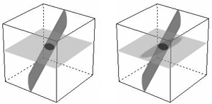
Ordinary projection techniques still present problems of visibility. Consider the case depicted on the left of Fig. 7. If a plane slices the path in the middle as shown, only an oval will appear on that plane. The rest of the path can only be revealed as we move the plane up and down but each time still is limited to just an oval. Instead, we want to see a longer portion of the path projected onto the plane, depicted on the right side of Fig. 7. The region of intersection should be most clearly visible, but the other regions should cast shadows onto the plane. Moreover, this effect should occur in all three viewing dimensions.

 

chen-cube-model
Figure 7 Projection without shadowing (left) and with shadowing (right).

A novel projection algorithm is developed to improve path visibility. Three new volumes $p_{i}(\vec{x})$, $p_{j}(\vec{x})$, and $p_{k}(\vec{x})$ equal in size to the original volume $p(\vec{x})$ are created, corresponding to the three viewing directions $\vec{i}$, $\vec{j}$, and $\vec{k}$. We now show the algorithm for projection along $\vec{i}$, which produces a set of $\vec{j}$-$\vec{k}$ slices, but the method is applied analogously along $\vec{j}$ or $\vec{k}$. The steps of the algorithm are:

1.

Volume $p_{i,low}(\vec{x})$ is filled with a dimmed version of $p(\vec{x})$, specifically $p_{i,low}(\vec{x}) = \alpha \cdot p(\vec{x})$, where we have used $\alpha = 0.5$. This serves as a background for the paths.

2.

Every path point's influence needs to be extended beyond the point's immediate location. A useful metric is the orthogonal distance between a point P and a plane D, which is defined as the distance between P and the point in D closest to P. For a $\vec{j}$-$\vec{k}$ slice located along $\vec{i}$ at x_s,i and a path point $\vec{x}_p = (x_{p,i}, x_{p,j},$ $x_{p,k}, \cdots)$, the closest point on the slice to $\vec{x}_p$ is $\vec{x}_s = (x_{s,i}, x_{p,j}, x_{p,k}, \cdots)$. 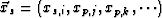Thus, the orthogonal distance is |x_p,i - x_s,i|. If this distance is small enough, then a scaled version of the data value at $\vec{x}_p$ in $p(\vec{x})$ should be shown at $\vec{x}_s$ in $p_{i}(\vec{x})$. Specifically, for all $\vec{x}_p$ on the path,

$$\begin{eqnarray} p_{i}(\vec{x}_s) &=& max\{ p_{i,fade}(\vec{x}_p) ,\: p_{i,low}(... ... (2\sigma_{i}^2)} , \ \sigma_{i} &=& \frac{R_{i}}{10} , \nonumber\end{eqnarray}$$ (7) (8)

where R_i is the range of the data volume along direction $\vec{i}$. The value $p_{i,fade}(\vec{x}_p)$ defined by Eq. 8 is the data value on the path from the original volume attenuated by a Gaussian fading factor. The fading factor decreases as the path point and the $\vec{j}$-$\vec{k}$ slice are separated farther. Eq. 7 sets a lower threshold for using the attenuated values.

3.

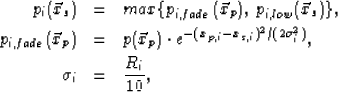
The previous step only covers projection at points $\vec{x}_p$ on the path and should be repeated for every point $\vec{x}_{pn}$ in the path neighborhood $N(\vec{x}_p,R)$ defined by Eq. 6. Redefine $\vec{x}_s$ to be the closest point on the 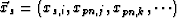$\vec{j}$-$\vec{k}$ slice to $\vec{x}_{pn}$: $\vec{x}_s = (x_{s,i}, x_{pn,j}, x_{pn,k}, \cdots)$. For all x_p on the path and for all $\vec{x}_{pn} \in N(\vec{x},R)$,

$$\begin{eqnarray} p_{i}(\vec{x}_s) &=& max\{ p_{i,fade}(\vec{x}_{pn}) ,\: p_{i,lo... ...(\vec{x}_{pn}) \cdot e^{-(x_{pn,i}-x_{s,i})^2 / (2\sigma_{i}^2)} ,\end{eqnarray}$$ (9) (10)

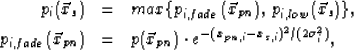
The variable radius R plays an interesting role here. There is one problem inherent in projection: loss of distance information along the direction of projection. Far and near portions of the path should be displayed differently on a plane of projection. The Gaussian fading in Eq. 10 helps in this regard, but a stronger indicator is needed. Towards this end, R is made to be a monotonically increasing function of the distance between the point $\vec{x}_{pn}$ and $\vec{x}_s$, the point on the $\vec{j}$-$\vec{k}$ slice closest to $\vec{x}_{pn}$.

$$\begin{eqnarray} R = \alpha R_i \cdot \sqrt{\frac{\vert x_{pn,i}-x_{s,i}\vert}{R_i}} ,\end{eqnarray}$$ (11)

where $\alpha = 0.2$ and R_i is again the range along direction $\vec{i}$. Since $0 \le \vert x_{pn,i}-x_{s,i}\vert \le R_i$, the square root term is between 0 and 1 and increases as $\vec{x}_{pn}$ and $\vec{x}_s$ are farther away. Therefore, on any plane of projection, distant parts of a path will appear dimmer due to Eq. 10 and thicker due to Eq. 11, while near parts of a path will appear undimmed and thinner. Recovery of distance information along the direction of projection is achieved.

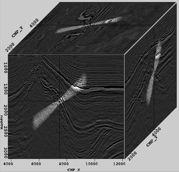
Fig. 8 shows projections onto slices in all three viewing dimensions for a path traversing a volume diagonally. As the projection radius grows and the projection intensity fades, the underlying path being projected is farther away from the current slice.

 

chen-pathview
Figure 8 Projection of a diagonal path onto orthogonal planes.