Interpolating a path from sample points

A path through a volume can be defined as a parametric curve $\vec{x}(t) = (x_1(t), x_2(t),$ $\cdots, x_M(t))$, where M is the number of dimensions and t is a free parameter.

In practice, though, what a user specifies is not a continuous $\vec{x}(t)$ but rather a finite, discrete set of vectors corresponding to points along $\vec{x}(t)$, say $\{ \vec{x_i} : 1 \le i \le N \}$. In each dimension $j \: (1 \le j \le M)$, a set $X_j = \{ (t_i, (\vec{x_i})_j) : t_i = i, 1 \le i \le N\}$ can be formed, where $(\vec{x_i})_j$ refers to the jth coordinate of vector x_i. So, from a set of N vectors, M sets each containing N parameter-coordinate pairs are obtained. Each X_j is correctly viewed as a discrete set of samples from the x_j(t), a scalar continuous function.

Recovering each x_j(t) from its samples X_j is a standard problem in interpolation. Assuming that the user has sampled densely enough so that there are no high-frequency oscillations for $\vec{x}(t)$ between samples, a good interpolating function for each x_j(t) can be constructed using a cubic spline Hou and Andrews (1978). A cubic spline is a curve that passes through the sample points and has continuous first and second derivatives. Thereafter, the interpolated curve can be sampled as densely as needed to give a good visual representation of the path.

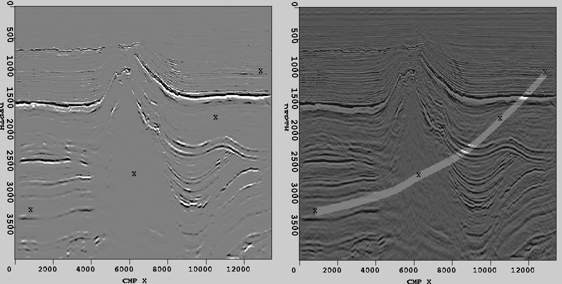
A very sparse set of starting samples is shown on the left of Fig. 6, marked with x symbols. Using cubic spline interpolation and then sampling at a higher rate, the curve shown on the right of Fig. 6 is obtained. The user only has to specify a minimal set of points, as few as two, to generate a path. In fact, Path View includes an algorithm, described in Section 3.3, to allow the user to input unordered points, such as first specifying two endpoints and then specifying a middle point.

 

chen-path-interp
Figure 6 Sample points (left) and interpolated path (right).