

Next: Conclusions
Up: Witten and Grant: Convex
Previous: Convex Optimization
125 CMP's from a 2-D prestack data set that was acquired in the Gulf
of Mexico were used. Since the Gulf of Mexico usually exhibits flat
reflectors, this is suitable for the Dix equation. The region is also
faulted which implies discontinuous velocities.
The approach taken for obtaining the RMS velocities is the same as
that in Valenciano et al. (2003), but will briefly be recreated
here. First, velocity analysis was preformed on each CMP. Then an
auto-picker was used to pick the maximum stacking power corresponding
to the best RMS velocity at each CMP position. An example velocity
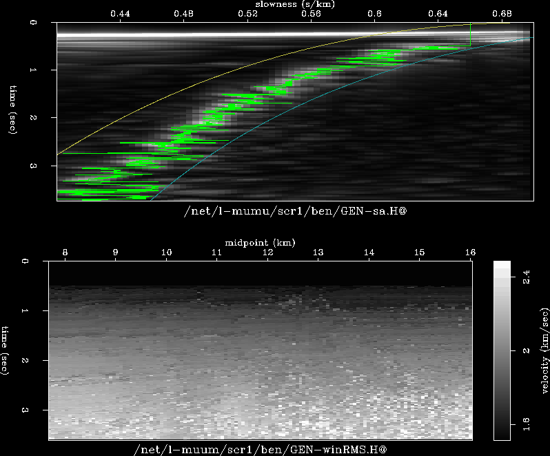
analysis with picks for a single CMP is shown on the top of Figure ![[*]](http://sepwww.stanford.edu/latex2html/cross_ref_motif.gif) . The
velocity values from all the CMPs can be combined to form a complete
RMS velocity model space. This is shown on the bottom of Figure
. The
velocity values from all the CMPs can be combined to form a complete
RMS velocity model space. This is shown on the bottom of Figure ![[*]](http://sepwww.stanford.edu/latex2html/cross_ref_motif.gif) .
Please note that the velocities picked in Figure
.
Please note that the velocities picked in Figure ![[*]](http://sepwww.stanford.edu/latex2html/cross_ref_motif.gif) are in
slowness rather than velocity, while the complete RMS model space is
in velocity. This is because the conjugate gradient method used a
slowness model, but the convex optimization failed with slowness and
velocity had to be used. This limitation may be because the values were all
close to forcing the solution down or due to the narrow range of
slowness values. Thus the images computed with conjugate gradients
were computed in slowness and inverted to velocity, while the convex
optimization images were computed directly with velocity values.
are in
slowness rather than velocity, while the complete RMS model space is
in velocity. This is because the conjugate gradient method used a
slowness model, but the convex optimization failed with slowness and
velocity had to be used. This limitation may be because the values were all
close to forcing the solution down or due to the narrow range of
slowness values. Thus the images computed with conjugate gradients
were computed in slowness and inverted to velocity, while the convex
optimization images were computed directly with velocity values.
vel-vrms
Figure 1 Top: Auto-picked RMS velocity of one CMP from a
2-D prestack dataset. Bottom: Raw RMS velocity map for all 125 CMPs


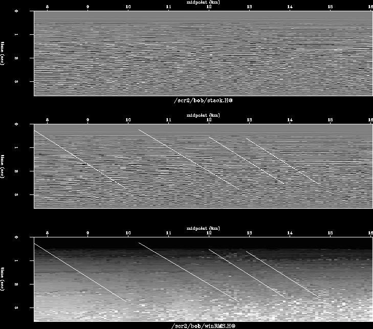
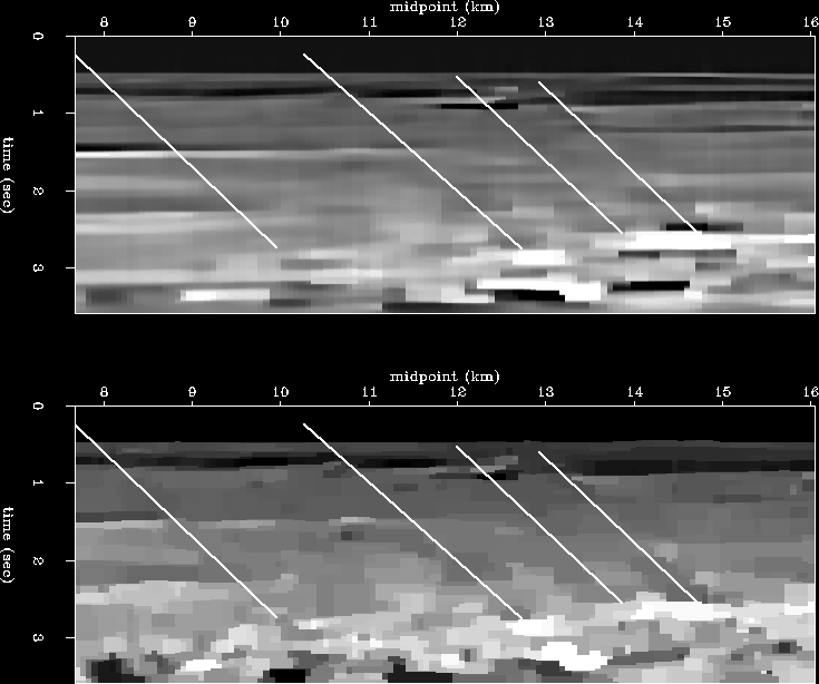
Figure ![[*]](http://sepwww.stanford.edu/latex2html/cross_ref_motif.gif) shows the stacked section which displays the
faulting mentioned above. The middle panel has the faults highlighted and the bottom
panels shows the same faults on the raw RMS velocity. It is
interesting to note that the raw RMS velocity shows the faults clearly.
shows the stacked section which displays the
faulting mentioned above. The middle panel has the faults highlighted and the bottom
panels shows the same faults on the raw RMS velocity. It is
interesting to note that the raw RMS velocity shows the faults clearly.
stack1
Figure 2 Top: Stacked data using the raw
RMS velocity. Middle: Stack data with lines showing the faults.
Bottom: RMS velocity with same lines showing the faults.


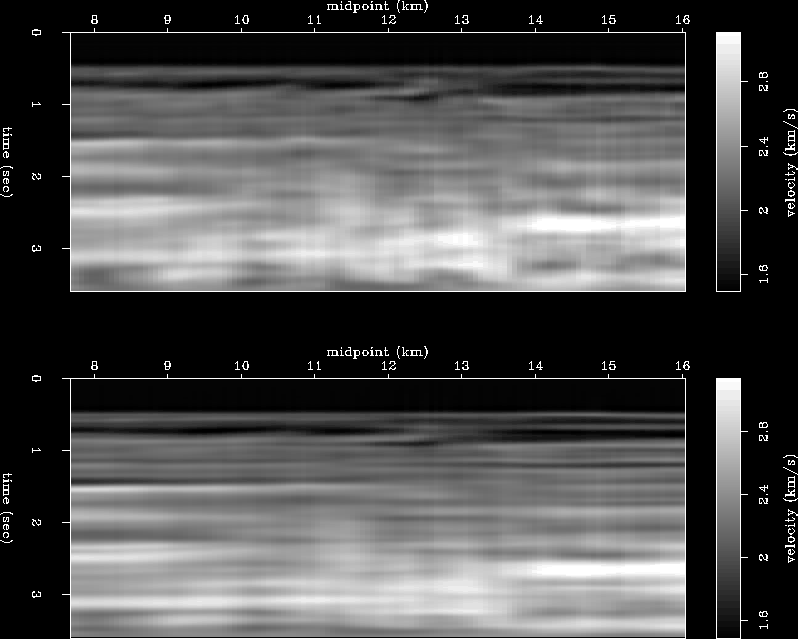
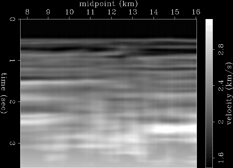
The top of Figure ![[*]](http://sepwww.stanford.edu/latex2html/cross_ref_motif.gif) shows the interval velocity resulting from
solving equations (2) with
shows the interval velocity resulting from
solving equations (2) with  regularization. The
bottom of Figure
 ![[*]](http://sepwww.stanford.edu/latex2html/cross_ref_motif.gif) shows the interval
velocity when equation (5) is solved with
shows the interval
velocity when equation (5) is solved with  regularization. Note that all interval velocities are clipped at
their respective maximums.
Both images in Figure
 ![[*]](http://sepwww.stanford.edu/latex2html/cross_ref_motif.gif) are very similar showing that convex optimization is at
least equivalent to conjugate gradients in terms of quality of
solution.
are very similar showing that convex optimization is at
least equivalent to conjugate gradients in terms of quality of
solution.
L2vint
Figure 3 Top: Interval velocity computed using conjugate
gradients with  regularization. Bottom: Interval velocity computed using convex optimization with
  regularization.


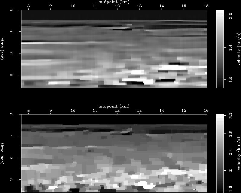
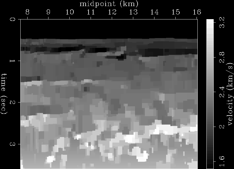
If we now look at the solutions to equations (2)
and (5) solved with a  regularization, shown in
Figure
 ![[*]](http://sepwww.stanford.edu/latex2html/cross_ref_motif.gif) , we can see that, as expected, a much blockier solution is
found. As in the previous figure,
the top panel of Figure
, we can see that, as expected, a much blockier solution is
found. As in the previous figure,
the top panel of Figure ![[*]](http://sepwww.stanford.edu/latex2html/cross_ref_motif.gif) , created by conjugate gradients, is very
similar to the bottom image, solved with convex optimization.
, created by conjugate gradients, is very
similar to the bottom image, solved with convex optimization.
L1vint
Figure 4 Top: Interval velocity computed using
conjugate gradients with  regularization. Bottom: Interval velocity computed using convex
optimization with
  regularization.


In the  regularization image, the faults do show up faintly.
If we overlay the same lines shown in Figure
 ![[*]](http://sepwww.stanford.edu/latex2html/cross_ref_motif.gif) onto
Figure
onto
Figure ![[*]](http://sepwww.stanford.edu/latex2html/cross_ref_motif.gif) , this becomes more obvious as shown in Figure
, this becomes more obvious as shown in Figure
![[*]](http://sepwww.stanford.edu/latex2html/cross_ref_motif.gif) . The faults may be
slightly more obvious in the problem solved with
. The faults may be
slightly more obvious in the problem solved with  , which is
blockier than with conjugate gradients. The difference in
``blockiness'' is due to the different
  's and how they are
applied in each case.
L1-interp
Figure 5 Same as Figure ![[*]](http://sepwww.stanford.edu/latex2html/cross_ref_motif.gif) except
with lines marking fault locations.
except
with lines marking fault locations.


There appears to be some low velocity anomalies near the bottom of the
interval velocity solution. This is predominately seen in the blocky
models, but there are uncharacteristically low velocities at late times
in all the models. As we can see from the stack in Figure
![[*]](http://sepwww.stanford.edu/latex2html/cross_ref_motif.gif) , there is no evidence to support such velocities. To correct this we can constrain the solution
further by adding bounds when solving the convex optimization
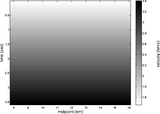
problem. If we assume that the interval velocity v(z) increases
linearly with depth:
, there is no evidence to support such velocities. To correct this we can constrain the solution
further by adding bounds when solving the convex optimization
problem. If we assume that the interval velocity v(z) increases
linearly with depth:
|  |
(7) |
then we can get a general estimate of the interval velocity. This is
shown in Figure ![[*]](http://sepwww.stanford.edu/latex2html/cross_ref_motif.gif) . Velocities 20 percent above and below
this model are used as the maximum and minimum constraints in equation
(6). Figures
. Velocities 20 percent above and below
this model are used as the maximum and minimum constraints in equation
(6). Figures ![[*]](http://sepwww.stanford.edu/latex2html/cross_ref_motif.gif) and
and ![[*]](http://sepwww.stanford.edu/latex2html/cross_ref_motif.gif) show the bounded constrained
show the bounded constrained  and
and  solutions,
respectively. As we can see, the low velocities occurring at late times
have been attenuated.
bounds
Figure 6 Model from which the upper and lower
velocity constraints are formed. Upper is  greater than this
everywhere and the lower is
  less.
less.


 L2vint-cvx-bounded
Figure 7 Solution by convex optimization with
 regularization and bound constraints.


 L1vint-cvx-bounded
Figure 8 Solution by convex optimization with
 regularization and bound constraints.


Next: Conclusions
Up: Witten and Grant: Convex
Previous: Convex Optimization
Stanford Exploration Project
1/16/2007
![[*]](http://sepwww.stanford.edu/latex2html/cross_ref_motif.gif) . The
velocity values from all the CMPs can be combined to form a complete
RMS velocity model space. This is shown on the bottom of Figure
. The
velocity values from all the CMPs can be combined to form a complete
RMS velocity model space. This is shown on the bottom of Figure ![[*]](http://sepwww.stanford.edu/latex2html/cross_ref_motif.gif) .
Please note that the velocities picked in Figure
.
Please note that the velocities picked in Figure ![[*]](http://sepwww.stanford.edu/latex2html/cross_ref_motif.gif) are in
slowness rather than velocity, while the complete RMS model space is
in velocity. This is because the conjugate gradient method used a
slowness model, but the convex optimization failed with slowness and
velocity had to be used. This limitation may be because the values were all
close to forcing the solution down or due to the narrow range of
slowness values. Thus the images computed with conjugate gradients
were computed in slowness and inverted to velocity, while the convex
optimization images were computed directly with velocity values.
are in
slowness rather than velocity, while the complete RMS model space is
in velocity. This is because the conjugate gradient method used a
slowness model, but the convex optimization failed with slowness and
velocity had to be used. This limitation may be because the values were all
close to forcing the solution down or due to the narrow range of
slowness values. Thus the images computed with conjugate gradients
were computed in slowness and inverted to velocity, while the convex
optimization images were computed directly with velocity values.
