Next: Table-driven implicit finite-difference migration
Up: Shan: Implicit migration for
Previous: Introduction
For isotropic media, the dispersion relation for the one-way wave equation can be represented as
|  |
(1) |
where  is the circular frequency, v=v(x,y,z) is the velocity, kz is the wavenumber,
 is the radial wavenumber, and kx, ky are wavenumbers for x and y respectively.
Let
is the radial wavenumber, and kx, ky are wavenumbers for x and y respectively.
Let  ,
and
,
and  .
The square-root function can be approximated by a series of rational functions:
.
The square-root function can be approximated by a series of rational functions:
|  |
(2) |
The coefficients  and
and  can be obtained by Taylor-series analysis or rational factorization.
If we consider the second-order approximation (n=1) and
can be obtained by Taylor-series analysis or rational factorization.
If we consider the second-order approximation (n=1) and  ,
,  ,we obtain the traditional
  equation. The coefficients and can
also be obtained by least-squares optimization, and a more accurate finite-difference scheme like
the
equation. The coefficients and can
also be obtained by least-squares optimization, and a more accurate finite-difference scheme like
the  equation can be obtained Lee and Suh (1985).
For VTI media, the true dispersion relation requires solving a quartic equation numerically Shan and Biondi (2005).
With the assumption that the S-wave velocity is much smaller than the P-wave velocity,
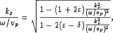
the dispersion relation for VTI media can be obtained analytically and represented as follows:
|  |
(3) |
where vp=vp(x,y,z) is the vertical velocity, and  and
and  are the
anisotropy parameters defined by Thomsen (1986):
are the
anisotropy parameters defined by Thomsen (1986):
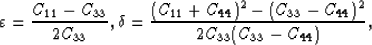
where Cij are elastic stiffness moduli.
Let  and
and  .
This dispersion relation can be further simplified under the weak anisotropy assumption, and
it can be approximated as
.
This dispersion relation can be further simplified under the weak anisotropy assumption, and
it can be approximated as
|  |
(4) |
where 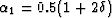 and
and 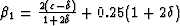 Ristow and Ruhl (1997).
The coefficients
Ristow and Ruhl (1997).
The coefficients  and
and  are obtained analytically by Taylor-series analysis.
As in the isotropic case, the coefficients and can also be obtained
by least-squares optimization. The advantage of least-squares approximation is that I do not have to derive an explicit approximated
expression for the dispersion relation analytically. This is especially useful for anisotropic media.
For VTI media, I can use the true dispersion relation, and no assumption of small S-wave velocity and weak anisotropy is necessary.
Generally, the Padé approximation suggests that
if the function 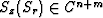 , then Sz(Sr) can be approximated by a rational function
Rn,m(Sr):
, then Sz(Sr) can be approximated by a rational function
Rn,m(Sr):
|  |
(5) |
where
and
are polynomials of degree n and m, respectively. The coefficients ai and bi can be obtained
either analytically by Taylor-series analysis or numerically by least-squares fitting.
kz1
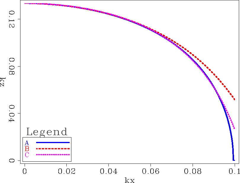
Figure 1 Dispersion relation: curve A is the true dispersion relation; B is the aprroximate
dispersion relation by Tayor-series analysis; C is the approximate dispersion relation by optimization.
|
|  |


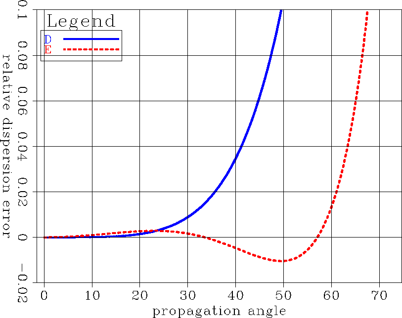
err1
Figure 2 Relative dispersion error: curve D is the relative dispersion error of the approximation by Taylor-series
analysis; E is the relative dispersion error of the approximation by optimization.
|
|  |
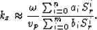
We can obtain the coefficients ai and bi by solving the following optimization problem:
|  |
(6) |
where  is the maximum optimization angle.
This problem can be changed to
is the maximum optimization angle.
This problem can be changed to
|  |
(7) |
The optimization problem (7) can be solved by a least-squares method.
Given  and
and  , we can solve ai and bi from equation (7), and
we can approximate kz as follows:
, we can solve ai and bi from equation (7), and
we can approximate kz as follows:
|  |
(8) |
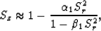
As Ma (1981) suggested, if m=n, equation (8) can be further split into a rational-function series as follows:
|  |
(9) |
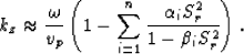
The dispersion error of approximation (9) is given by
| ![\begin{displaymath}
\Delta k_z=\frac{\omega}{v_p}\left[\sqrt{\frac{1-(1+2\vareps...
..._{i=1}^{n}\frac{\alpha_iS_r^2}{1-\beta_i S_r^2}\right)\right]. \end{displaymath}](img37.gif) |
(10) |
The relative dispersion error is defined by  .
.
For the second-order approximation (m=1,n=1), Figure ![[*]](http://sepwww.stanford.edu/latex2html/cross_ref_motif.gif) shows the true and approximated dispersion relation, given
shows the true and approximated dispersion relation, given  and
and  .
In Figure , curve A is the true dispersion relation curve. B is the approximated dispersion
suggested by Ristow and Ruhl (1997), in which
.
In Figure , curve A is the true dispersion relation curve. B is the approximated dispersion
suggested by Ristow and Ruhl (1997), in which  and
and  . C is the approximated dispersion
relation by the least-squares optimization, in which
. C is the approximated dispersion
relation by the least-squares optimization, in which  and
and  .
The dispersion relation by optimization (C) approximates the true dispersion relation better than
the approximation using Taylor-series analysis and the weak anisotropy assumption.
.
The dispersion relation by optimization (C) approximates the true dispersion relation better than
the approximation using Taylor-series analysis and the weak anisotropy assumption.
Figure shows the relative dispersion error. D is the relative dispersion error
of the approximation using the Taylor-series analysis. E is the relative dispersion error of the optimized one-way
wave operator. Figure shows that opimization greatly improves the dispersion relation.
If we accept a one-percent dispersion error, the optimized one-way wave-equation
is accurate to  while the approximation using Taylor-series analysis is accurate to only
  .
.
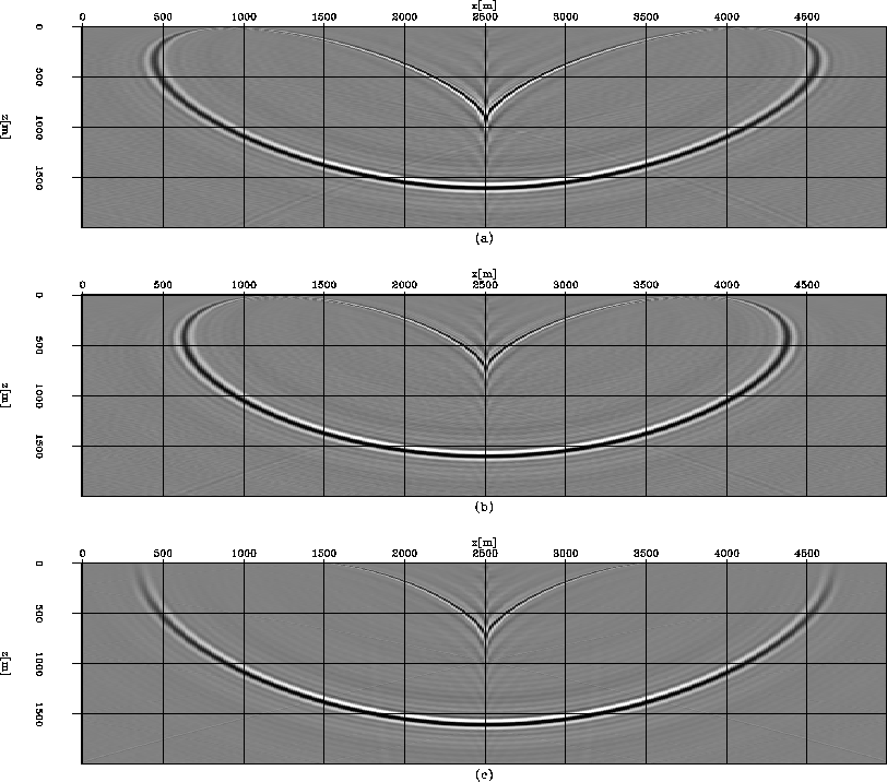
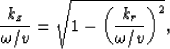
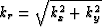
impulse
Figure 3 Impulse responses: (a) Optimized finite-difference method;
(b) Finite-difference method by Tayor-series analysis; (c) Phase-shift method.
Next: Table-driven implicit finite-difference migration
Up: Shan: Implicit migration for
Previous: Introduction
Stanford Exploration Project
4/5/2006