Results

To increase the sampling by an integer factor, a PEF is typically estimated on the input data. In this example with a large gap, this will not suffice. Instead, we estimate the PEF on the pseudo-primaries generated by equation 1 using equation 3 and then use that PEF to interpolate the recorded data with equation 4. The results of this experiment are shown in Figure .

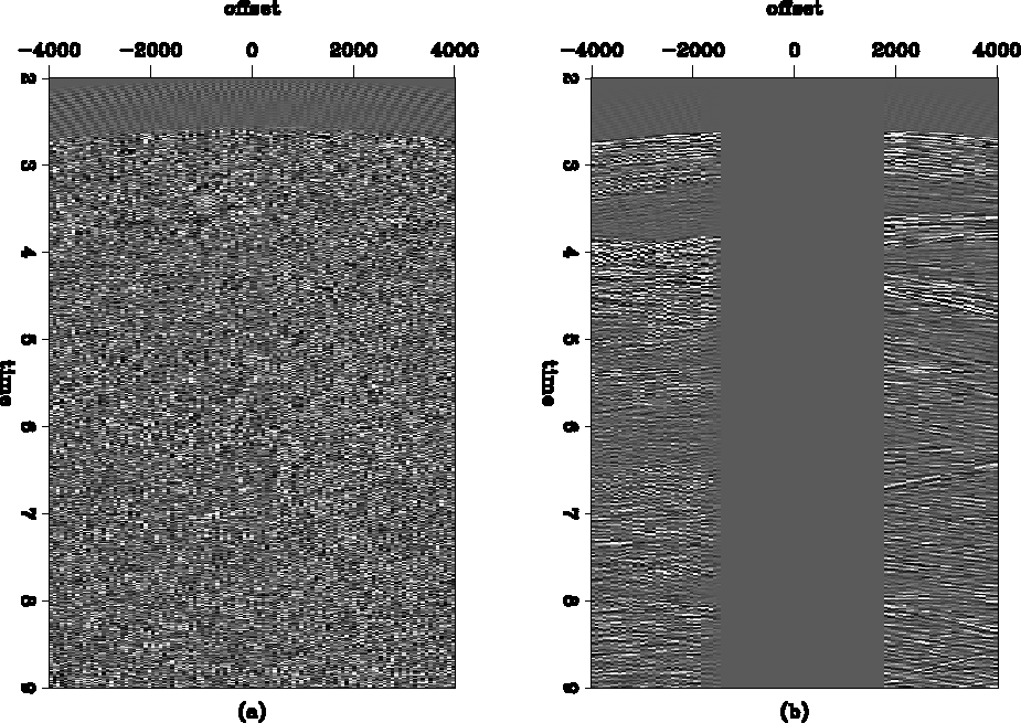
The near offset gap is 4000 feet or 53 traces, as shown in Figure (a). The complete data in Figure (b) is used as input to equation 3 with Figure (a) as input to equation 4, which produces Figure (c), which illustrates that if we estimate the PEF on the answer we can perfectly recreate the data. Figure (d) shows the main result of this paper, which is when the pseudo-primaries are used as input to equation 3.

 

resid
Figure 3 (a) PEF estimated on pseudo-primaries convolved with pseudo-primaries. (b) PEF after convolution with input data.

The results in Figure (d) are promising, but not ideal. Most of the events are successfully continued through the data, but some interference is present. One method to quality control the PEF estimation is to examine the residual of the estimation of equation 3. If this result is uncorrelated and low in amplitude, the PEF has captured all of the useful information in the pseudo-primaries. Similarly, the PEF can then be convolved with the recorded data, with the output shown in Figure .

Figure (b) shows that while the PEF estimated on the pseudo-primaries does a good job of whitening the recorded data, the result is not ideal, unlike Figure (a) where the PEF is convolved with the pseudo-primaries. Differences in spectral content of the data are the most obvious cause, and any adjustments to this algorithm can be quality controlled by looking at this intermediate result.