Subsurface-offset Hessian

The prestack migration image (subsurface offset domain) for a group of shots positioned at ${\bf x}_s=(x_s,y_s,0)$ and a group of receivers positioned at 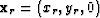${\bf x}_r=(x_r,y_r,0)$ can be given by the adjoint of a linear operator ${\bf L}$ acting on the data-space ${\bf d}({\bf x}_s,{\bf x}_r;\omega)$ as

$$\begin{eqnarray} {\bf m}({\bf x},{\bf h}) &=& {\bf L}'{\bf d}({\bf x}_s,{\bf x}_... ...\sideset{}{'}\sum_{{\bf x}}{\bf d}({\bf x}_s,{\bf x}_r;\omega), \end{eqnarray}$$ (7)

where ${\bf G}({\bf x},{\bf x}_s;\omega)$ and ${\bf G}({\bf x},{\bf x}_r;\omega)$ are the Green functions from shot position ${\bf x}_s$ and receiver position ${\bf x}_r$ to a model space point ${\bf x}=(x,y,z)$, and ${\bf h}=(h_x,h_y,h_z)$ is the subsurface offset. The symbols $\sideset{}{'}\sum_{{\bf h}}$ and $\sideset{}{'}\sum_{{\bf x}}$ are spray (adjoint of the sum) operators in the subsurface offset and model space dimensions, respectively.

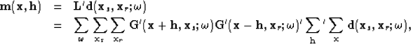
The synthetic data can be modeled (as the adjoint of equation 7) by the linear operator ${\bf L}$ acting on the model space ${\bf m}({\bf x},{\bf h})$ with ${\bf x}=(x,y,z)$ and ${\bf h}=(h_x,h_y)$

$$\begin{eqnarray} {\bf d}({\bf x}_s,{\bf x}_r;\omega)&=&{\bf L}{\bf m}({\bf x},{\... ...\bf x}_s}\sideset{}{'}\sum_{\omega} {\bf m}({\bf x},{\bf h}), \end{eqnarray}$$ (8)

where the symbols $\sideset{}{'}\sum_{{\bf x}_r}$,$\sideset{}{'}\sum_{{\bf x}_s}$, and $\sideset{}{'}\sum_{\omega}$ are spray operators in the shot, receiver, and frequency dimensions, respectively.

In equations 7 and 8 the Green functions are computed by means of the one-way wave equation Ehinger et al. (1996) and the extrapolation is performed using the adequate paraxial wave equations (flux conservation) Bamberger et al. (1988).

The quadratic cost function is

$$\begin{eqnarray} S({\bf m}) &=& \frac{1}{2} \sum_{\omega}\sum_{{\bf x}_s}\sum_{{... ...f d}({\bf x}_s,{\bf x}_r;\omega)-{\bf d}_{obs} \right], \nonumber \end{eqnarray}$$ (9)

while its first derivative, with respect to the model parameters ${\bf m}({\bf x},{\bf h})$, is

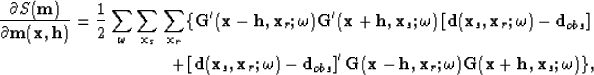$$\begin{eqnarray} \frac{\partial{S({\bf m})}}{\partial{{\bf m}({\bf x},{\bf h})}}... ...f x-h},{\bf x}_r;\omega) {\bf G}({\bf x+h},{\bf x}_s;\omega) \}, \end{eqnarray}$$ (10)

and its second derivative with respect to the model parameters ${\bf m}({\bf x},{\bf h})$ and ${\bf m}({\bf x'},{\bf h'})$ is the subsurface offset Hessian:

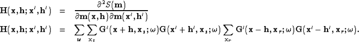$$\begin{eqnarray} {\bf H}({\bf x,h};{\bf x',h'})&=& \frac{\partial^2{S({\bf m})}... ...f x}_r;\omega) {\bf G}({\bf x'-h'},{\bf x}_r;\omega). \nonumber \end{eqnarray}$$ (11)

The next subsection shows how to go from subsurface offset to reflection and azimuth angle dimensions following the Sava and Fomel (2003) approach.