Next: Data space vs. Image
Up: Example
Previous: Data Space
We now apply adaptive subtraction after migration.
We perform split-step wavefield
downward-continuation
migration to go from the data to the image space. Both the original seismic
data and the multiples model were migrated with the same algorithm. Because the velocity model is
still an unknown at this stage of the processing, we use a simple, vertical-gradient velocity function.
We use the same velocity model for the original data set and the multiples model.
Since this particular data set corresponds to an OBC acquisition, both the original data set and
the multiples model were re-datumed in order to have both sources and
receivers at the same depth level before the migration.
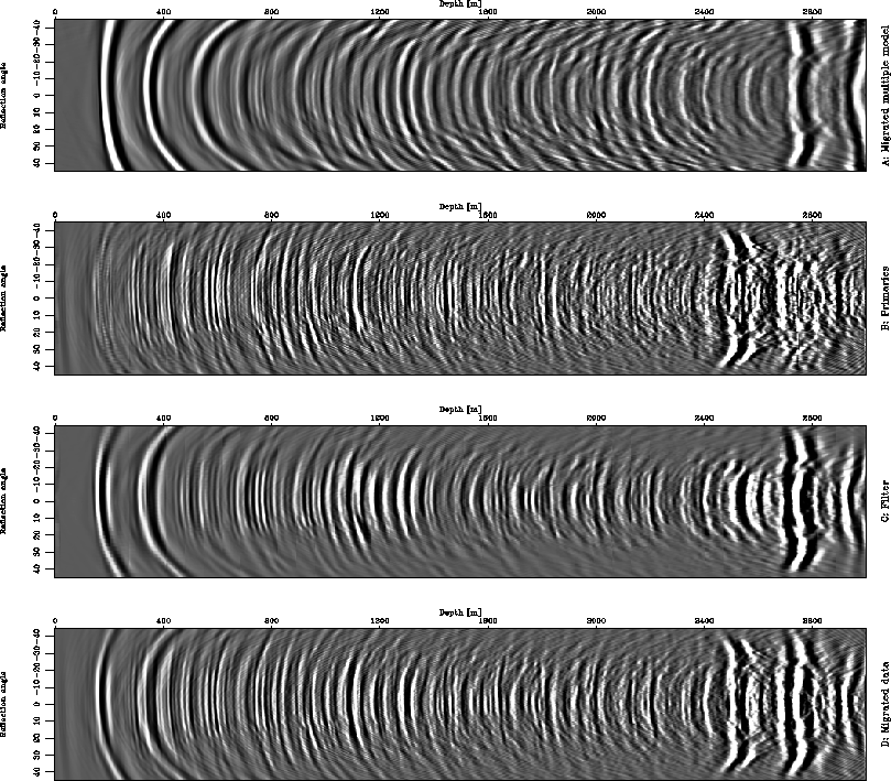
Figure ![[*]](http://sepwww.stanford.edu/latex2html/cross_ref_motif.gif) shows one angle-domain common-image gather,
following the same presentation scheme for the results in the data space. The figure
shows, from top to bottom: A) the migrated multiples model; B) the result of adaptive subtraction
in the image space, that is the primaries; C) the filter obtained with the migrated multiples model
for performing the subtraction; and D) the migrated data set.
shows one angle-domain common-image gather,
following the same presentation scheme for the results in the data space. The figure
shows, from top to bottom: A) the migrated multiples model; B) the result of adaptive subtraction
in the image space, that is the primaries; C) the filter obtained with the migrated multiples model
for performing the subtraction; and D) the migrated data set.
We first observe that both the migration of the entire data set and the migration of the multiples
(panels A and D) have a residual curvature in the angle gathers because we have the
correct velocity model. However, this is not an obstacle to performing
the multiples subtraction in this
domain, since both panels present the same residual moveout.
After estimating the filter for performing the subtraction (panel C), we were able to eliminate
almost all the multiples present in our multiples model.
ispace_4panel
Figure 4 Image space multiple removal. From top to
bottom: A) Migrated multiple model; B) Primaries; C) Filter; D) Migrated data.


Next: Data space vs. Image
Up: Example
Previous: Data Space
Stanford Exploration Project
5/3/2005