


Next: Synthetic Test: Data Interpolation
Up: Theory of noise attenuation
Previous: Sparse inversion
Applying a mask in equation (6) eliminates the contribution
of the empty traces in the model space, making them invisible to the
inversion. Therefore, by simply remodeling a data panel from
the estimated model  after inversion without the mask,
the missing traces are reconstructed. Then, the interpolated data
vector
after inversion without the mask,
the missing traces are reconstructed. Then, the interpolated data
vector  can be estimated as follows:
| 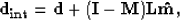 |
(9) |
where I is the identity matrix. Now, for the noise removal, we
simply (1) apply a mute  in the radon domain that isolates and
preserves the signal, and (2) transform the muted panel in the data
space as follows:
in the radon domain that isolates and
preserves the signal, and (2) transform the muted panel in the data
space as follows:
| 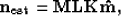 |
(10) |
where  is the estimated signal (specular reflections and impinging source).
The estimated noise (diffracted energy and ambient noise) is
obtained by subtracting the estimated signal from the input data:
is the estimated signal (specular reflections and impinging source).
The estimated noise (diffracted energy and ambient noise) is
obtained by subtracting the estimated signal from the input data:
|  |
(11) |
Note that the estimated noise and signal in equations (10) and
(11) are for the non-interpolated data. To compute the
estimated noise and signal for the interpolated data, M must be removed
in equations (10) and (11) and d must be
replaced by in equation (11).
Next: Synthetic Test: Data Interpolation
Up: Theory of noise attenuation
Previous: Sparse inversion
Stanford Exploration Project
5/3/2005