Computing the traveltime: an example

We will illustrate the theory presented above using the multiple reflection event S1010201G (the zeros denote the Earth surface). For this event, n=6, 1 less than the total number of bounces in the earth. The first step is generating sequences $\phi_i$ and l_i, according to (5) and (6):  

$$\left\{\phi_1,\phi_2,\phi_3,\phi_4,\phi_5,\phi_6,\phi_7\righ... ...1,\theta_0,\theta_1,\theta_0,\theta_2,\theta_0,\theta_1\right\}$$ (39)

and  

$$\left\{l_1,l_2,l_3,l_4,l_5,l_6,l_7\right\}=\left\{d_1,d_0,d_1,d_0,d_2,d_0,d_1\right\}$$ (40)

We prepend $\phi_0=-\frac{\pi}{2}$ to the sequence of angles, then we compute the $\beta$ sequence:

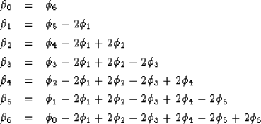$$\begin{eqnarray} \beta_0&=&\phi_6 \\ \beta_1&=&\phi_5 - 2 \phi_1 \\ \beta_2&=&... ... - 2 \phi_1 + 2 \phi_2 - 2 \phi_3 + 2 \phi_4 - 2 \phi_5 + 2 \phi_6\end{eqnarray}$$ (41) (42) (43) (44) (45) (46) (47)

It may be useful to notice the regularities in signs and indices. The summation and trigonometric operators in (25) and (26) can be written in matrix form to verify the correctness of their numerical implementation. We then compute the auxiliary vectors given by (29) and (33):  

$$\begin{array} {l} {\bf u}_1 = \frac{2}{v}l_5\left[ {\begin{... ...i_7} \\ {-\cos\phi_7} \\ \end{array}} \right] \\ \end{array},$$ (48)

 

$${\bf u}_4=\frac{1}{v}\left[ {\begin{array} {*{20}c}{\sin\le... ...cos\left(-\beta_6\right)+\sin2\phi_7} \\ \end{array}} \right],$$ (49)

For our very particular case in which some of the bounces are with the surface (d₀=0, $\theta_0=0$),  

$${\bf u}_1 = \frac{2}{v} d_1\left[ {\begin{array} {*{20}c}{+... ...-\cos\left(2\theta_1-\theta_2\right)} \\ \end{array}} \right],$$ (50)

 

$${\bf u}_4=\frac{2}{v}\cos\left(3\theta_1+\theta_2\right) \le... ...{-\sin\left(\theta_1+\theta_2\right)} \\ \end{array}} \right],$$ (51)

and the traveltime for each offset h can now be computed by plugging these vectors directly into (35). By performing trigonometric operations, we may find that the expression for the distance is the same as that in Equation (A-14) of Levin and Shah (1977).