


Shuey (1985) showed that in a 1-D earth, the measured reflection strength of an event at the surface is approximately linear with the square of its incidence angle, at angles less than 30 degrees. In a 1-D earth, the NMO equation gives an approximate relationship between offset and incidence angle. Claerbout (1995) defines the ``stepout'', p, as the spatial derivative of an event's traveltime curve:
| |
(37) |
![[*]](http://sepwww.stanford.edu/latex2html/cross_ref_motif.gif) . In a 1-D earth, the
traveltime curve of a primary reflection is approximately given by the NMO
equation (). Taking the derivative of equation () with
respect to offset, then substituting into equation () gives the
following expression for the sine of incidence angle as a function of offset:
. In a 1-D earth, the
traveltime curve of a primary reflection is approximately given by the NMO
equation (). Taking the derivative of equation () with
respect to offset, then substituting into equation () gives the
following expression for the sine of incidence angle as a function of offset:
 |
(38) |
), at which point the AVO ``slope'' and ``intercept''
parameters may be estimated, usually via a linear least-squares fit to the
data after resampling from offset to
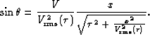
Figure illustrates the estimation of AVO slope and
intercept parameters on a deep reflector in the Green Canyon 3-D data, before
and after application of LSJIMP. The reflector, which is well under the
multiples in the data, is denoted on the zero offset section with ``O'' symbols.
The maximum amplitude in a small time window around the reflection were picked
automatically, and make up the input data to the least-squares estimation.
 |
We see that while the parameter estimates contain the same trends before and
after LSJIMP, the LSJIMP result is more consistent and less ``noisy'' across
midpoint. My implementation of LSJIMP works on a CMP-by-CMP basis, so the
results shown in Figure are not smoothed across
midpoint. The similarity across midpoint is an expression of the true lithology
- lithology which LSJIMP better reveals.
Figure illustrates, as a function of midpoint, the
small time windows taken around the deep reflector shown in Figure
, before and after LSJIMP. The input data to an AVO
parameter estimation are picked maximum amplitudes within the time window as a
function of ![]() . Notice the significant increase in reflector
clarity after LSJIMP. Also recall that the data residuals (e.g., in Figures
and )
are quite small. Therefore, the cleaner reflection events after LSJIMP in
Figure are not only better for AVO analysis - they
also fit the recorded data in a quantitative fashion. LSJIMP is not an ad
hoc post-processing technique.
. Notice the significant increase in reflector
clarity after LSJIMP. Also recall that the data residuals (e.g., in Figures
and )
are quite small. Therefore, the cleaner reflection events after LSJIMP in
Figure are not only better for AVO analysis - they
also fit the recorded data in a quantitative fashion. LSJIMP is not an ad
hoc post-processing technique.
 |
, before and after LSJIMP. Individual panels along
the vertical axis correspond to windows taken at different midpoint locations.
Left: Data windows before LSJIMP. Right: Data windows after LSJIMP.


